1. Home
2. / Market Reports

Zillow’s Open Market Home Price Appreciation Forecasting Methodology

By lisabo on 25 Jan 2022

What drives open market house price appreciation? Where will it be in a month or in a year? How about seasonal effects? Why do otherwise similar homes in some markets appreciate at different rates than in other areas? 

Truly understanding the housing market requires a firm understanding of these questions – and existing forecasting methods proved insufficient at Zillow. So, we created new approaches to forecasting that more directly and accurately address these challenging but critical questions.

Traditional forecast approaches suffer from many well-known problems. First of all, home price growth can be non-stationary over longer periods of time given structural breaks in the economy, which makes it harder to build models that will generalize out of sample, in the future. Second, many traditional, ARIMA-type models tend to be backward-looking: They expect the future to look like the past. 

At Zillow, we needed something more suited to adapt to volatile and unprecedented market conditions, so we created our own approach that corrects for several of these problems. In particular, we pioneered an approach that greatly corrects for nonstationarity on the regional level, and also has the added benefit of enabling us to use local forward-looking features in our models – rather than backward-looking features such as the recent trend in a market.

What drives housing prices?

So, what drives house price appreciation? We start with the following questions around existing structural relationships: How do demand and supply interact to affect house prices? And how do we model demand and supply? How do we best model home price appreciation on the national level, while still being able to accurately forecast what is happening on the regional level – within larger areas like metros, and also much smaller areas including ZIP codes and neighborhoods? Understanding what impacts national and regional housing market dynamics helps guide us in what relationships to expect – and, critically, what features could be the most important leading indicators of future home price appreciation.

National HPA is driven by a slew of macro factors that affect for-sale inventory and home sales, including mortgage rates, the overall health of the economy, home affordability, household formation and new home completions. In addition to modeling the national dynamics, we want to model local (regional) dynamics in a way that can help capture why some regions experience very rapid growth in a very short time – HPA in Austin, for example, was 22% in the three-month span from February-April 2021 – and others grow more slowly or not at all.

National HPA forecasting and regional forecasting are separate tasks. Zillow’s national model captures macro economic factors in a short-term and long-term model, whereas the regional dynamics are driven by local leading indicators.

A tiered approach to modeling the dynamics of the housing market

Traditional forecast approaches suffer from many well-known problems. First of all, home price growth can be non-stationary over longer periods of time given structural breaks in the economy, which makes it harder to build models that will generalize out of sample, in the future. Second, many traditional, ARIMA-type models tend to be backward-looking: They expect the future to look like the past. At Zillow, we needed something more suited to adapt to volatile and unprecedented market conditions, so we created our own approach that corrects for several of those problems. In particular, we pioneered an approach that greatly corrects for nonstationarity on the regional level, and also has the added benefit of enabling us to use local forward-looking features in our models, rather than backward-looking features such as the recent trend in a market.

To this end, we employ a two-tiered approach, where we first strip out the national component from the regional home price appreciation index, in order to obtain local residual regional time-series. This methodology helps us in several ways. First, such residuals are highly stationary since any macro trend is by definition stripped out of them. Second, these residuals capture isolated local idiosyncratic movements for which  we can discover features that predict these movements. In addition, we focus on creating the best national HPA forecast that we can, utilizing macro factors in addition to any leading indicator features that might be relevant at that level.

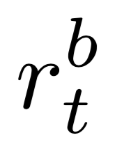
The national home appreciation index growth rate is denoted by HPA_n.  Regional HPA indices growth rates are denoted by HPA_r, for r in all MSAs under consideration. Regional residual appreciation growth  is calculated as 

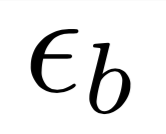
The β parameters represent the historical relationship between regional growth and national growth for each region. The parameters are determined via pooled regressions with shrinkage toward the mean of all individual betas. 

Because macro trends are stripped out, the residual regional growth time-series are stationary and represent idiosyncratic growth patterns for each region (Figure 1). These residuals form the basis for our targets in the modeling process — in other words, the things we are trying to predict. 

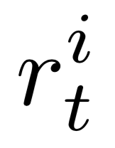
We form targets for each MSA that are constructed as the change in the residuals over horizons h, in h = 1,…,12 months. For each horizon, we will build a forecasting model for each MSA’s regional residual growth over that horizon. Since these residuals represent idiosyncratic behavior, we choose to model them using a seasonality term and unpooled regressions on a set of leading features. The output of the model created at a given time t is a forecasted residual growth for each horizon, , for the period t+h in the future.

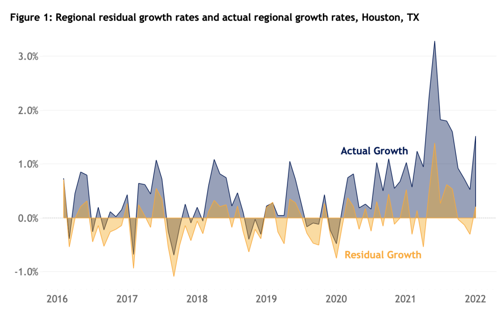
Figure 1: An example of regional residual growth time-series (orange) versus actual regional growth (for Houston, TX  MSA). The residual time-series is stationary, mean-reverting around 0 in the long run, whereas the time-series of actual growth-rates is not.

In addition to creating forecasts on the residuals, we also need to forecast the national growth of HPA_n over horizons h, in h = 1,…,12 months. Once we have the national forecasts and the residual regional MSA forecasts, we create the final regional MSA forecasts at a certain time t for the periods t+h in the future by putting everything back together:

Finally, to get forecasts on the ZIP code level, we attribute the MSA level forecasts to each ZIP code, according to the historical correlation of a given ZIP code’s rate of home value growth to that of its parent MSA.

In the next sections, we will cover first the construction of the regional models, then details of the national model. 

A simple structural model

At the regional level, we need to model unique local (regional) dynamics that can help capture why home values in some regions grow faster or slower than in others. We start with a toy model for a region and assume that, relative to the national level, each region has its own supply and demand equilibrium driven by local dynamics. Specifically, demand is considered to be the total number of active buyers, while supply is the total number of active sellers (for-sale inventory). Local changes in supply and demand could be driven by factors including net migration into a region, local demographics (in particular the volume of people at or near the typical home-buying age) and/or the relative affordability and general appeal of a region (especially considering current opportunities for remote work).  Because any/all of these factors could be leading indicators of future local demand and supply, it is important to measure them in a timely manner.

Supply is defined as the number of active sellers, or for-sale inventory, following the dynamics  

Where:

•   is the for-sale inventory at the start of time t
•   is the number of homes bought during the time interval t
•   represents new listings and new construction that enter the market during the time interval t
•   captures people who removed their homes from the market
•   are other unaccounted for factors (for example, natural disasters that destroy homes)

Demand is defined as the number of active buyers, and evolves according to 

Where:

•   is the number of buyers at time t
•   is the number of home buyers who bought homes at time t
•   represents new buyers at time t
•   is the number of active buyers deciding to drop out of the market
•   are other, unaccounted-for factors.

More specifically, new buyers can be decomposed as  

Where:

•  represents net migration into the region
• denotes new buying population from within the region (including those aging into their prime home buying years, or renters who have saved up enough money to buy a home)
• captures speculators and other investors

The next question is, how does demand and supply relate to the price?  To understand this we look at market tightness, defined as . Intuitively, if Θ is much greater than 1, we expect nonlinear feedback into the price, via bidding wars etc., that can result in a rapid rise in home price appreciation. Similarly, if is much smaller than 1, we can expect a rapid decrease in housing prices. Hence, we postulate with γ > 1, which is consistent with prior research that found prices should increase nonlinearly in Θ.¹

From our toy model,  after ignoring the unaccounted for factors  , we obtain:

implying that if we could measure all the variables in this ratio at time t, then we would have a leading indicator for market tightness  — and hence HPA — at a later time t+1.  

Feature selection 

We use the toy model above to help inform what type of features we should focus on to model regional residual dynamics, guided by our main hypothesis that market tightness (Θ) directly affects home prices. The task then is to design features that can be leading indicators of regional demand (active buyers), supply (active sellers) or market tightness directly.  

Potential leading indicators we are exploring include, again: Net migration into a region, local demographics, and the relative affordability and general appeal of a region. Our current forecasting model utilizes proprietary Zillow data to gauge demand, including (among other things) how many buyers are interested in a given home (measured by the number of times users choose to contact an advertised agent via the home listing after viewing the home online) and how many days a home spends on the market before an offer is accepted and the home goes pending. 

The term for example, which describes active buyers at time t, could be approximated by counting how many user/agent contacts there are in a region. We also construct and examine other proprietary measures of buying interest, including a “market hotness” metric, defined in part as the share of homes gone pending in 7 days or less. 

Supply (inventory) is easier to directly measure — we know how many homes are currently listed for sale on the market (with new construction being an additional element). Currently,  is very well measured by the for-sale inventory that we observe on the market. 

Based on these features, the final form of the regression that we employ for each MSA r is:

Where:

• Θ:  market tightness leading indicator proxy (eg contacts /Inventory)
• ρ:  share of homes gone pending in 7 days or less
• σ:  seasonality factor (target encoded by month of year)

The national model

We build forecasting models for 1 month-, 3 months- and 12 months-ahead cumulative seasonally adjusted HPA growth, interpolate growth rates in between, and overlay the seasonal factor prediction for each horizon to generate non-seasonally adjusted forecasts. 

Short-term model

The short-term forecast for the seasonally adjusted HPA growth is an ensemble of a direct forecasting model and an error correction model. The direct forecasting model is a linear regression model to predict HPA growth using a feature that captures national market tightness Θ, following the same motivation as on the regional level, that this quantity is relevant and leading for HPA. Specifically, we are using a feature related to the median value of views per listing across the top 500 MSAs. The error correction model (ECM) aims to exploit the mean reverting property of deviations of HPA to underlying fundamental valuations. There are two stages in the ECM model. 

In stage 1, we run a cointegration regression between the accumulated growth rate and the months’ supply of homes available (defined as inventory/sales) and rate shocks – defined as the negative three-month moving average of 30-year, fixed mortgage rates net of its long-term average. In stage 2, we model the acceleration rate, defined as the change in HPA growth rate using the latest one-month acceleration rate and the error term from step 1. The acceleration rate yields a much more stationary time series to work with, and the error term can capture the deviation of actual HPA from the fundamental value implied from the above economic features. Finally, we forecast the seasonal component by  removing the trend mean value and cycle mean value from the historical growth rate. The final forecast is the sum of the leading indicator forecast, the ECM forecast and the seasonality forecast.

Long-term model

The long-term forecast is an ensemble of the ECM and the median, annualized monthly HPA growth over the past 4 years. The long-term ECM model is similar to the short-term model, but with more contemporaneous features in the second-stage regression, where we use Zillow’s internal homes sales and inventory forecasts to obtain a proxy for forecasted months’ supply. We then employ an interpolation scheme using the short-term and long-term forecasts to obtain forecasts of cumulative growth for each horizon  h, in h = 1,…,12 months.

The model training process

We have developed a time-safe back-testing framework used for model evaluation, allowing us to run historical simulations. Assume we start the simulation at some time-point τ in the past. For each forecast horizon, we only use data prior to τ, train the models, and make forecasts of the future growth rate over the horizon h. The next month, we repeat this process, all the way up to a predetermined time . We then compare the forecasts that we made with what actually occurred, and can gather performance statistics including mean error and mean absolute error. We utilize a similar framework with bootstrapping across the universe of MSAs to obtain distributions that help us decide if a feature is statistically significant or not.

Accuracy and performance

The index that we use to measure home price appreciation in this example is Zillow’s debiased ZHVI index.² However, the approach can be applied to any home price appreciation index without loss of generality. Below we exhibit performance statistics for the top 100 MSAs, based on a backtest over the time period beginning in January 2019 through November 2021. This model has been in production since September 2021.

Table 1: Panel Forecast Accuracy

Table 1: Forecast accuracy summarized across time and top 100 MSAs in a back-test from January 2019-November 2021.

Acknowledgments: We thank Luca Silvan Becker for contributions to the Forecasting Framework and Infrastructure.

¹ In a 2019 paper by Alina Arefeva, an auction model is developed that theoretically determines the sales price as a function of active buyers and active sellers, and specifically as a function of market tightness.
²The debiased Zillow Home Value Index (ZHVI) takes Zillow’s headline, publicly available ZHVI and utilizes a control factor to modify growth rates based on actual repeat sales.