1. Home
2. / Policy & Industry
3. / Fair Housing

Using a Oaxaca Decomposition to Dissect the Relationships Between Wealth, Homeownership & Race

By Cody Fuller on 12 Oct 2015

Previously, we’ve examined the complicated relationship between race and real estate, analyzing how race can color the path to homeownership and the ways in which it might be harder for black households to become homeowners. We’ve also investigated the relationship between homeownership, race and wealth.

Because purchasing a home is one of the easiest ways for a family to build wealth, it’s natural to wonder how lower homeownership rates among blacks might explain persistent differences in wealth between blacks and other races. It’s also worthwhile to ask how much of those gaps can be explained by differences in education, income and demographics, and how much is attributable to more pernicious causes.

To further understand the interaction of these complex dynamics, we developed a methodology to help us answer these questions, utilizing a so-called “Oaxaca Decomposition,” named after University of Arizona professor Ronald Oaxaca.

How does it work? Read on.

Two-Way Oaxaca Decomposition

The goal of a two-way Oaxaca decomposition is to explain the difference in means between two different groups in terms of explained and unexplained portions of the difference. The explained portion is the portion that can be explained by observable differences in socioeconomic conditions, like differences in income, education etc. The unexplained difference is that which cannot be explained by differences in socioeconomic conditions, or largely unobservable differences, like differences in individual preferences or differences in the underlying process of wealth accumulation by different groups.

The first step in this process is to run a regression for the different groups, in this case blacks and whites, with the dependent variable being the natural log of wealth and the independent variables. These variables include:

• • Year of Survey
  • Homeownership Status
  • Log of Income
  • Age of Household Head
  • Marital Status of Household Head
  • Number of Children in Household

Number of Adults in Household

• Wealth Status of Parents
• Inheritance

 

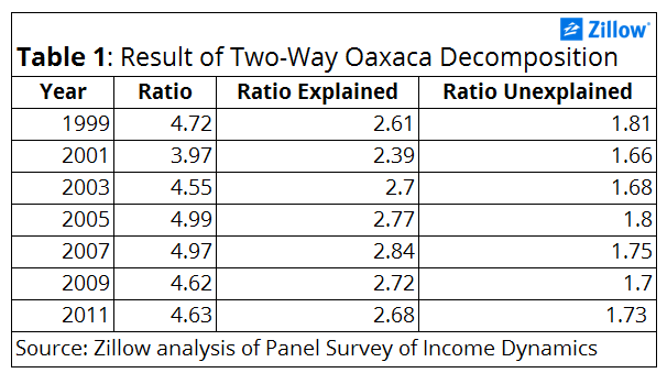
We run these separate regressions to obtain estimates b_w and b_b regression coefficients for the whites and blacks. Now we can characterize the difference in log wealth in the following way:

ΔlnWealth = Δx’b_w + x_b‘ΔbWhere Δx’b_w is the explained portion, and the unexplained portion is x_b‘Δb. We then exponentiate, and the left side of the equation becomes an estimate of the (geometric) mean of the wealth ratio.

From here, we can summarize the results in table 1. However this no longer has the nice simple linear interpretation, it becomes multiplicative, so the ratio is the product of the explained and the unexplained parts of the ratio. In other words if there was no unexplained difference, a difference in coefficients, we would expect the wealth ratio to be 2.68 in 2011 as opposed to 4.63.

But this is not the question we set out to answer. We want to know, controlling for select socioeconomic characteristics, what the effect the different propensities of blacks and whites to purchase homes has on their wealth. In order to do this, we need to be able to estimate the probability of owning a home, given socioeconomic characteristics, for only whites. We will use these synthetic probabilities in a new two-way Oaxaca decomposition to see how much the difference in wealth is impacted by different propensities to purchase homes.

Probability Model

Our previous research estimated the following model:

P(Owning a Home|White, Socioeconomic Characteristics) = γWhere the select socioeconomic characteristics are as follows:

• Year of Survey
• Log of Income
• Age of Household Head
• Marital Status of Household Head
• Number of Children in Household
• Number of Adults in Household
• Wealth Status of Parents
• Inheritance
• Education of Head
• Education of Wife
• Couple Status of Head
• Number of Vehicles

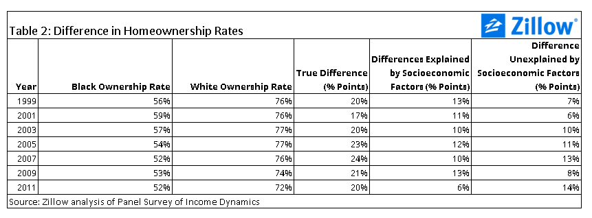
We randomly selected 80 percent of the data to estimate the model, and reserved the rest for testing. Out-of-sample accuracy was approximately 81 percent.

We use the estimate to produce the results in table 2:

Here, we see that if blacks had the same propensity to purchase homes as whites, black homeownership would be 14 percentage points higher.

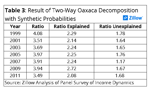
Two-Way Oaxaca Decomposition with Synthetic Probabilities

Now we can leverage these probability estimates to understand how they impact wealth accumulation for whites and blacks. Let x_b be the mean of the explanatory variables for blacks. Replace the mean homeownership rates from the data with our synthetic estimate γ and let this new vector be x_b,γ. We then repeat the original two-way Oaxaca Decomposition using x_b,y instead of x_b:

ΔlnWealth* = (x_w – x_b)’b_w) + x_b,y‘ΔbWhere ΔlnWealth* is the difference in mean log wealth when we use our synthetic probability estimates. Using this, we are able to replicate the table from the first section, except with synthetic probabilities (table 3):

Probably the biggest difference is that we see the wealth ratio should have decreased if blacks had the same propensity to purchase homes as whites. But only looking at the means of the wealth ratio can be difficult to interpret. Table 4 has the cash explanation:

So, in 2011, if blacks purchased homes at the same rate as whites, controlling for socioeconomic characteristics, average wealth for blacks would be roughly 33 percent higher.

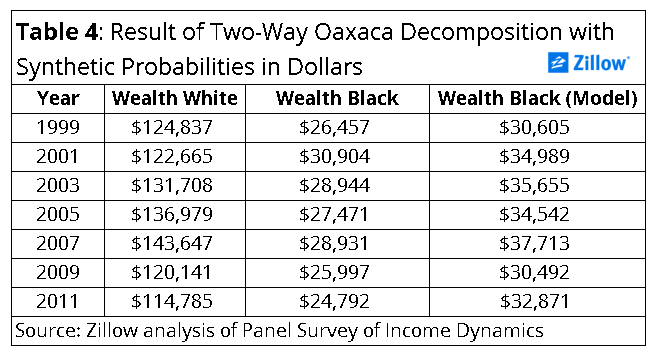
For model-fitting reasons, those without wealth or income were excluded from this analysis. Additionally, the top 1 percent of income earners and wealth holders were also eliminated from this analysis.