The number of homes available to buy, the number of home sales that can ultimately occur and the amount of time homes spend on the market before selling are all interconnected. Understanding the relationship between these factors can help us understand how the housing market is thriving despite limited inventory, and why the market as a whole may be resetting to a lower baseline for “normal” inventory levels.

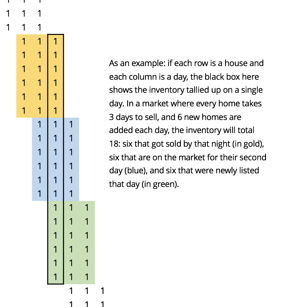
Time on market and inventory fit together in a (relatively) simple relationship that we can put into an equation. First, it’s helpful to start by defining inventory and where it comes from. When we tally up the inventory of active listings at the end of day t, we know the total comes from the inventory already on the market one day ago (at t-1), plus whatever new listings that came on that day, minus the homes that were sold (or de-listed, but for simplicity we’ll consider those sold, since the end-result is the same — a listing previously on the market is no longer):

Another way of getting at a home’s chance of selling is to describe it as the inverse of each home’s average days on market: For instance, in a market where a home has a 1 in 20 chance of selling on any given day, homes will average 20 days on the market. Substituting this in, we see that:

This way of representing the flow of sales shows how pending sales volume (the most immediate measure of sales, which leads actual, closed sales volume) is proportional to the pool of inventory — and, critically, that proportion varies with how fast homes are selling.

We can think of the average probability of selling as the velocity in the market:

If the velocity is equal to one, homes sell instantaneously. Then:

Rearranging this equation shows that, on average, the total count of Sales each day will equal the inventory level times the daily probability that each home on the market will sell:

The Steady State

Typically, the level of inventory ebbs and flows over the year because the annual peak in new listings is somewhat out of sync with the yearly peak in sales. But if we imagine a year in which inventory ends up exactly where it started the year, we can logically conclude that in the aggregate, sales (plus de-listings) matched new listings. 

This would be a steady-state scenario for inventory over the course of a year, and it would imply we can substitute new listings (which get observed much sooner than sales) into the above equation, dropping the time period indicators because this is now an approximate relationship that holds true over a long, aggregated period of time:

In such a steady-state scenario, we can actually use the flow of new listings and data on the seasonal pattern of days on market to project what inventory path would be consistent with them:

To show how closely this approximates reality, consider a very simple model of a market that begins in a steady, high-inventory state. Suppose this market experiences a shock that raises daily pending sales 20% higher than before, but with no change to the flow of new daily listings. In this situation, overall inventory must fall, along with the average number of days on market. Multiplying the unchanged level of new listings by the falling average number of days on market very closely approximates the actual path of falling inventory. 

If, eventually, new listings rise to match pending sales, then total inventory will stabilize at a new, lower level.