Zillow’s Zestimate forecast is a forecast of the change in an individual property’s Zestimate over the next 12 months.  The Zestimates themselves are a time series of Zillow’s estimated home value for a particular property over time. More information on Zestimates can be found here. The forecasts are our best prediction for the Zestimate of a particular home one year from now, given the data that is currently available. These forecasts will not have a direct impact on the Zestimate in 12 months, which incorporates any relevant new data between now and then.

Methodology

To forecast a path for the individual Zestimate, we rely on two different types of data. The first is the county level Zillow Home Value Forecast which forecasts the Zillow Home Value Index (ZHVI) and is produced using a variety of economic and housing data. The forecast is combined with data on the individual characteristics of the property, including its features and the past behavior of its Zestimate. This methodology section will concentrate on how those aggregate forecasts, in combination with property characteristics, are used to construct the forecast for a particular property. Broadly, the forecast is constructed by first forming a prediction for the Zestimate one year from now (a point forecast), which is then interpolated to construct a path for the Zestimate between now and then.

Point Forecast

Several academic papers have documented that certain segments of the housing market display more volatility than others, even at very specific geographic levels. For example, Guerrieri, Hartley and Hurst (2010), looking at zip code level data, document that areas on the boundaries of rich neighborhoods are the most price sensitive (rising most during booms and falling most during busts), while Landvoigt, Piazzesi and Schnieder (2013) document in San Diego that individual homes in poorer neighborhood appreciated fastest during the run up of the housing bubble. Based on these findings, we model the appreciation for individual properties as:

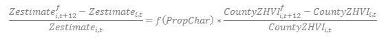
Where Zestimate_i,t denotes the current Zestimate for a particular property i, and Zestimate^f_i,t+12 denotes our prediction for the Zestimate of that property in 12 months. Taken together, the left hand side of this equation is the predicted percentage appreciation of the specific property. Similarly, CountyZHVI_i,t is the current ZHVI for the county in which the property resides, while CountyZHVI^f_i,t+12 denotes our prediction for the ZHVI of that county in 12 months.
The function f(PropChar) specifies how we expect an individual property’s Zestimate to perform relative to the county’s ZHVI as a function of the individual characteristics of a property. To specify the function f(PropChar) we first define:

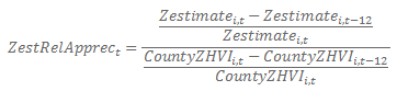
Then the function f(PropChar) is specified as follows:

f(PropChar)=α+β*HedonicCharacteristics+γ*ZestRelApprec_t
Where HedonicCharacteristics refers to a vector of housing characteristics and includes the number of bedrooms, bathrooms, finished square footage and if the home is on the higher or lower end of properties in the area. If, for example, in a region where one bedroom homes have tended to vary quite sharply with the market while four-bedroom homes tend to be less volatile in a given region, the estimation might suggest that a particular one-bedroom property might be expected to appreciate or depreciate twice as much as the rest of the county they are in, whereas a particular property with four bedrooms might be expected to appreciate or depreciate half as much as the county as a whole. ZestRelApprec_t is the rate of appreciation (or depreciation) the home has experienced in the past year relative to the county as a whole. A large body of academic work (for example Case and Shiller [1989]) has found evidence for momentum in housing prices – homes which rise (fall) in value one year are more likely to rise (fall) again the next year. This is already incorporated into how Zillow constructs its forecasts at the county level, but including past appreciation in our specification for f(PropChar) allows us to capture this feature for individual homes. The coefficients in this equation are estimated cross-sectionally using data from the prior year.

Forecast Path

Having computed the predicted Zestimate in 12 months for a property, the path for the Zestimate is interpolated using a cubic spline, which smoothly connects the forecasted value to the current value of the Zestimate. As a guard against over-fitting, this spline is then shrunk towards the forecast for the county as a whole, with the shrinkage weights gradually declining over time.

Geographical Coverage and Historical Forecast Accuracy

Currently the Zestimate forecast is available for more than 50 million individual properties spanning 550 counties across the United States. The predictive accuracy of these one-year forecasts was assessed by back-testing the model over the past five years. Back-testing consists of running forecasts on historical data where the forecasted value is produced from out-of-sample data. The below table summarizes the average absolute percentage error of the 12-month forecast. The average is taken over all properties. This forecast error is compared to a naive forecast based on a simple random walk model, and to simply extending our county forecast to individual properties. The construction of a property-specific forecast significantly improves accuracy.

Model	Average Absolute % Error	Improvement over Naïve
Naïve Forecast	7.35%	0%
County Forecast	6.47%	11.9%
Zestimate Forecast	5.84%	20.5%

 

References

Case, Karl E. and Shiller, Robert J. (1989), “The Efficiency of the Market for Single-Family Homes” The American Economic Review
Guerrieri, Veronica and Hartley, Daniel and Hurst, Erik, (2013), “Endogenous Gentrification and Housing Price Dynamics” Journal of Public Economics
Landvoigt, Tim and Piazzesi, Monika and Schnieder, Martin (2013), “The Housing Market(s) of San Diego” NBER Working Paper 17723

Updated March 11th 2014 by Krishna Rao