Methodology: Zillow Observed Rent Forecast (ZORF)

Beginning in November 2024, Zillow has released the Zillow Observed Rent Forecast (ZORF). ZORF provides forecasts for the Zillow Observed Rent Index (ZORI), which measures changes in asking rents over time. ZORF is currently available at the national level for two categories: single-family residences (SFR) and multifamily residences (MFR).
Rental prices and the rental market are inherently interconnected with the for-sale real estate market. To effectively capture the relationship between these two markets, and to leverage our industry-leading, for-sale market forecasting suite in ZORI forecasting, we pioneered a structural approach grounded in solid economic theory and well-supported by empirical evidence.
We first found that the month-over-month (MoM) growth of SFR ZORI, as a measure of single-family rental price appreciation, and the MoM growth of the Zillow Home Value Index (ZHVI), as a measure of home value appreciation for typical homes, are co-integrated on a seasonally adjusted basis (Chart 1). In forecasting, co-integration refers to a unique statistical property where two non-stationary time series tend to stay in sync or follow a similar path over time. As shown in Chart 1, despite short-term fluctuations, there is a stable, long-term co-movement between SFR ZORI and ZHVI. Specifically, when one moves too far away from the other, they tend to “pull” back toward each other, eventually ensuring the two remain in sync.
Chart 1: Single-Family ZORI and ZHVI, US, Seasonally Adjusted MoM Growth
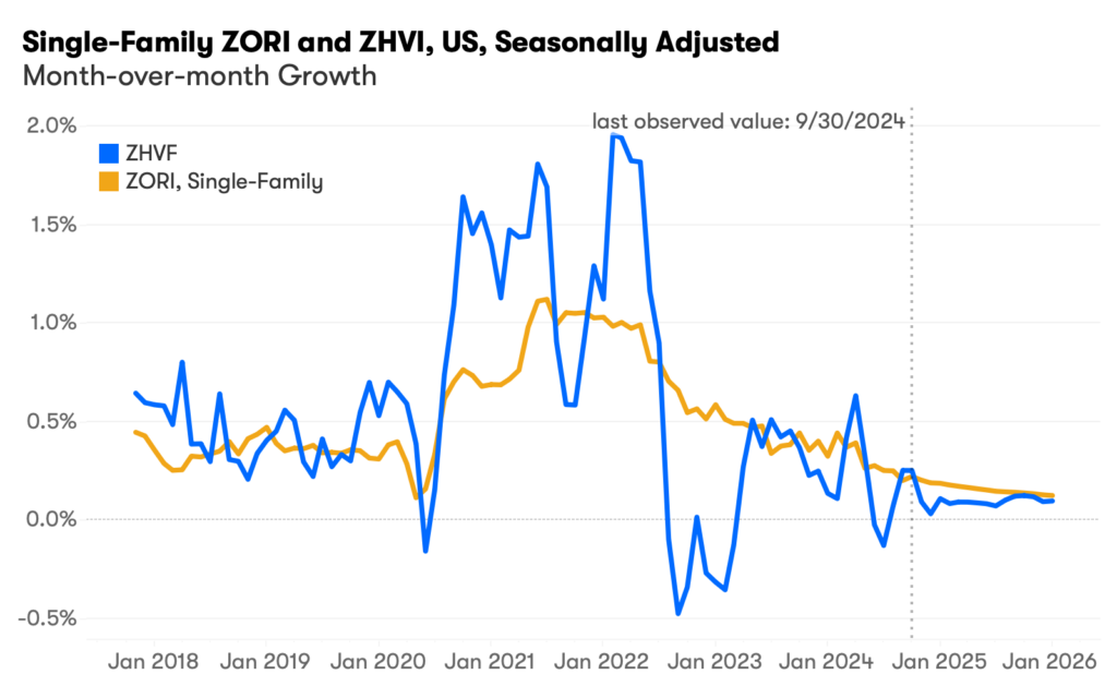
Rental prices and home values are co-integrated because there are economic driving forces from both the demand and supply sides that ensure a pull towards long-term equilibrium. In other words, for-sale and rental markets are substitutes for each other for both the mover and the homeowner and / or landlord. So when one market changes, tradeoffs between them change.
On the demand side, households are constantly weighing the “rent versus buy” decision by comparing the cost of renting to the cost of buying a home. On the supply side, landlords of single-family homes have the flexibility to either lease out or sell their properties based on market conditions. These forces work together to ensure the co-movement of SFR ZORI and ZHVI in the long run.
Let’s say there was an expected increase in home price appreciation from a previous month. On the demand side, when home prices rise beyond rents – and so too the monthly payments as a new owner — households are pushed toward renting a home rather than buying. This in turn puts upward pressure on rents until the markets are balanced again (or something else unexpected happens). On the supply side, landlords would be incentivized to sell their properties and put that new price premium to work earning interest in some other investment, instead of renting out the home. As a result, an upward momentum in ZHVI in the for-sale market leads to increased demand and reduced supply in the rental market, ultimately driving stronger SFR ZORI growth. Similarly, a negative shock to ZHVI would correspondingly lead to weaker growth in SFR ZORI.
As single-family and multifamily living are themselves substitutes, there is also co-integration between SFR ZORI and MFR ZORI (Chart 2). Renters are continually weighing the trade-offs between renting a single-family home and renting a unit in a multifamily property. This demand-side force ensures that rental prices for the two types of housing cannot deviate indefinitely. However, because multifamily properties don’t have the same sales liquidity as single-family rentals that can more easily take advantage of price shocks in the for-sale market, price volatility is more pronounced and longer lived for multifamily.
Chart 2: Single-Family and Multifamily ZORI, US, Seasonally Adjusted MoM Growth
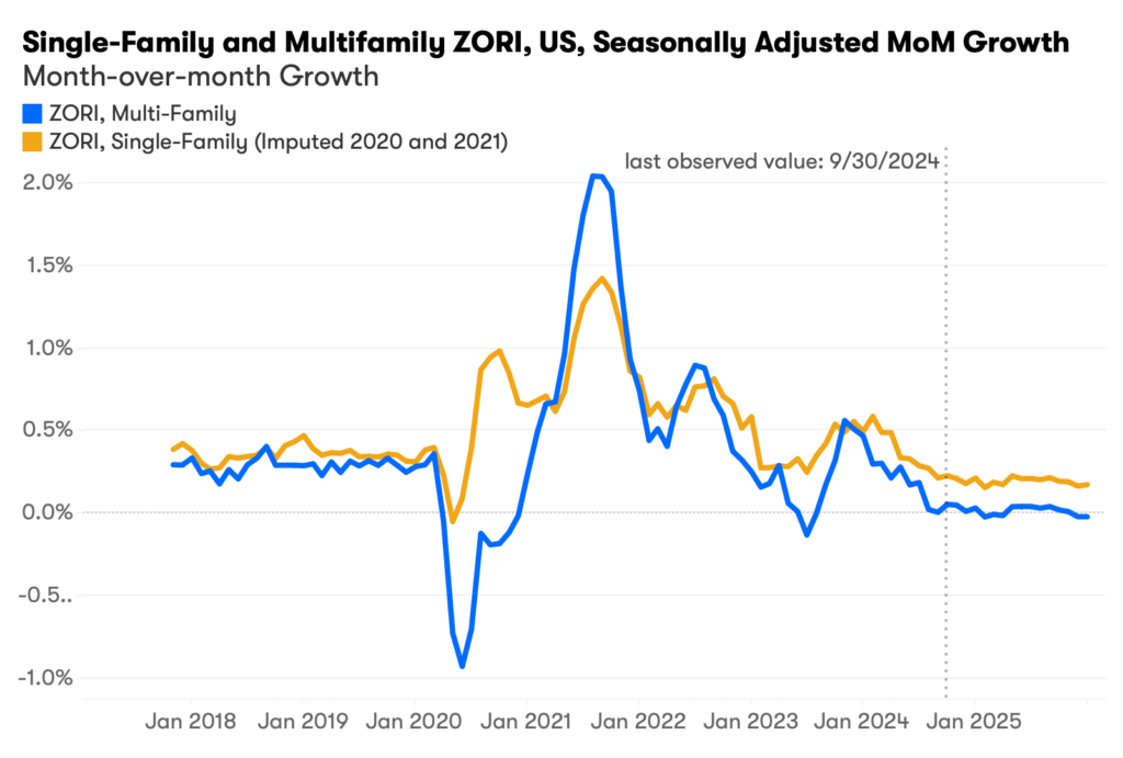
* A different seasonal adjustment method is employed in Chart 2 than Chart 1
We performed the Johansen test on both pairs of time series. The statistical test results confirmed that there is indeed a co-integration relationship between SFR ZORI and ZHVI, as well as between SFR ZORI and MFR ZORI.
We then built two error correction models (ECM) to leverage both co-integration relationships: first, we forecast the SFR ZORI using ZHVI, and then we forecast MFR ZORI using SFR ZORI.
An error correction model is a two-stage regression that simultaneously models long-term and short-term processes. In Stage 1, we run a co-integration regression to capture how the seasonally adjusted MoM growth rates of the feature and the target co-move. That is, Stage 1 quantifies the long-run relationship. Stage 2 measures the short-run relationship and, in particular, the rate of return towards the long-run relationship any time the two series diverge. This is done by calculating how the rate of change of our ZORI target is affected by deviations from the long-run relationship (as proxied by the errors from Stage 1). Essentially, there are two driving forces for forecasts in ECM: the trend in the feature itself and the extent to which the target deviates from the long-term equilibrium determined by the feature. The specification for the two ECM models is:
SFR ZORI model:
![]()
![]()
MFR ZORI model:
![]()
![]()
α, the error correction coefficient, indicates the speed of correction towards equilibrium and is estimated to be negative in both models. Note that in the MFR ZORI model, we introduced a constant β0 in Stage 1 to capture the consistently stronger growth of SFR ZORI compared to MFR ZORI, along with a dummy variable set to 1 for the pandemic months of 2020 to account for the pandemic-related shocks that disproportionately impacted MFR ZORI growth.
We use the ECM to iteratively forecast the seasonally adjusted MoM growth rates from 1 to 24 months ahead. We then add back a forecasted seasonality factor, derived from past years’ seasonality, to obtain non-seasonally adjusted MoM growth rate forecasts. From these, we derive cumulative growth rates and level forecasts.
We performed a time-safe backtest to evaluate the model forecast accuracy. Starting at a time point t in the past, we only use data available prior to t to train the ECM and make ZORF forecasts using forecasted ZHVI (i.e., ZHVF). We repeat this process for each subsequent month until t = August 2024. We then compare the ZORF generated in this exercise with the actual observed ZORI, and measure performance using root mean square error (RMSE) of cumulative growth rate. Table 1 presents the RMSEs for both SFR ZORF and MFR ZORF, along with the mean of cumulative growth as a reference. For instance, for 3-month ahead cumulative growth in SFR ZORF, our forecasts, on average, deviate from the mean of 2% by ±0.5%.
Table 1: ZORF Accuracy, Cumulative Growth
| SFR ZORF | ||
| RMSE | Reference: Cumulative Growth Mean | |
| 1-month ahead | 0.2% | 1% |
| 3-month ahead | 0.5% | 2% |
| 12-month ahead | 2.8% | 8% |
| MFR ZORF | ||
| 1-month ahead | 0.2% | 1% |
| 3-month ahead | 0.9% | 2% |
| 12-month ahead | 5.2% | 7% |
