In the Transaction & Engagement Analytics team at Zillow, our mission is to use data to uncover new strategic directions and optimize ongoing initiatives. We are the owners and stewards of metrics around customer interactions, including connections, when a home buyer or seller is connected with a real estate professional through Zillow, and transactions, when an individual goes on to buy or sell a home with the real estate professional they connected with through Zillow. We are often interested in the transaction rate, or the proportion of all interactions between consumers and agents beginning on Zillow that end with a home being bought or sold, i.e. transactions / connections.

While it may seem a trivial matter of counting the transactions and the connections, in practice there are several interesting data challenges. These encompass the larger topics of record linkage, censoring, and dealing with small data volumes. The challenge of estimating rates when we have limited amounts of data often arises when analyzing a particular dimension, such as an individual zip code or individual Zillow partner (e.g. real estate agent). To address this challenge, we use Bayesian statistical methods.

In this blog post, we will give a brief overview of three concepts of Bayesian statistics that are important to our work:

1. Conjugate priors
2. Empirical Bayes
3. Hierarchical models

First, let’s elaborate on one of the challenges.

The Challenge

We often want to calculate the transaction rate and similar metrics in various dimensions for which we have limited data. 

Take geography as an example. There is a single, nationwide rate that is calculated using all data collected over a period of time. This gives us a large number of observations so we can make very precise estimates.

But we may also be interested in geographic variance — how does one state, zip code or neighborhood differ from another? When comparing across these dimensions, we need to consider that we have collected different amounts of data for each, and so our estimates have varying degrees of precision. Furthermore, we may have a small number of observations for certain dimensions, such as a rural zip code, an individual neighborhood, or a new Zillow partner.

So while we have a lot of information on the overall distribution, we may have very limited information in certain specific dimensions that we are interested in. We’d like a method that allows us to use the information at the highest level (e.g. nationwide) to inform our estimates on the lowest level (e.g. individual neighborhood). This is where Bayesian methods come in.

Bayesian Methods at High Level

Bayesian inference allows us, through the application of Bayes’ rule, to quantify our uncertainty about an unknown parameter of interest, Θ. We do this through the use of a “prior,” which we consider a random variable following a probability distribution, π(Θ). The likelihood function, or the probability of the data (Y) given the parameters (Θ), is given as f(Y|Θ).

Though the application of Bayes’ rule: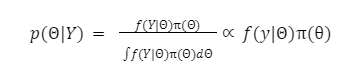

We calculate the p(ΘΙY), or the posterior distribution, as a product of the likelihood and the prior distribution. Note that ∝ here means proportional to, and what we are doing there is removing a normalizing constant that is difficult to calculate in practice. See a text on Bayesian inference for more details. 

Conjugate Priors

A prior and a likelihood pair are conjugate if the resulting posterior is a member of the same family of distributions as the prior. We’ll introduce this idea through our particular analysis problem, which is to estimate the unknown transaction rate (a proportion) of an individual zip code (which is a sample out of a population of zip codes).

Let Θ ∈ [0,1] be the proportion of connections in a zip code that transact through Zillow. We assume this proportion varies across zip codes following a Beta(α,β) distribution, θ∼ Beta(α,β). The Beta distribution’s support is (0,1), and it is a very flexible distribution, and so is a good choice for modeling proportions. The probability density function (PDF) of a Beta distribution is: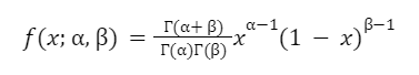

If we take a sample of connections from a particular zip code, we assume that the number of connections that transacted, Y ∈ {0,1,…,,n} is distributed following a binomial distribution, or Y|θ Binomial(n,θ), which has probability mass function: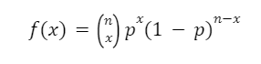

In our case, we are only interested in the terms that involve x, and so can drop:We can already see that the two previous functions resemble each other. Combining these, i.e. applying Bayes rule by the taking the product of the likelihood and the prior: 

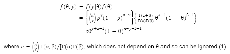
We can see that this results in another Beta distribution. This is our definition of the conjugacy given above; the resulting posterior distribution is the member of the family of distributions as the prior (Beta). 

The Wikipedia page for “Conjugate prior” states: “A conjugate prior is an algebraic convenience, giving a closed-form expression for the posterior; otherwise numerical integration may be necessary. Further, conjugate priors may give intuition, by more transparently showing how a likelihood function updates a prior distribution.”

The second part of that statement makes a data scientist’s life easier, as it lets us communicate the results in terms of pseudo-observations.

Pseudo-observations

As data scientists, a large part of our job is to clearly communicate to a non-technical audience, building trust and confidence in our solutions and recommendations. While the why behind conjugate priors involves some math, as we’ve just seen, the intuition behind what it means for our stakeholders is very easy to grasp. To see this, consider the mean of the prior distribution:

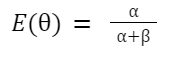
And the mean of the posterior distribution for a particular zip code:

We can see that the posterior mean is simply the prior mean with the number of success (y, or in our case, transactions) and number of observations (n, or in our case, connections) added. This leads us to the concept of pseudo-observations — α can be considered the prior number of transactions, while α + β can be considered the prior number of connections. This allows us to communicate what we doing in intuitive ways, such as:

• “We ‘start off’ a zip code with y transactions and n connections, and add to this as we learn more.
• “A zip code’s mean is the weighted average of the nationwide average and the data collected for that particular zip code.”

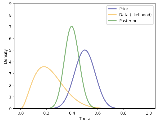
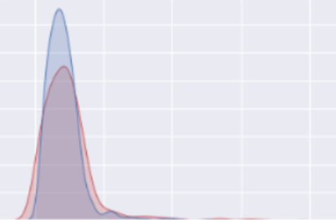
We can also build intuition through a visualization like the one below. This shows visually how the data (likelihood) combined with the prior results in the posterior (in the typical Bayesian terminology, we say that the likelihood has “shrunk” toward the prior):

Empirical Bayes

The next concept that is often useful is Empirical Bayes, which is when we use the data to set the priors. 

In the case of our beta binomial model for a proportion, i.e. zip-level transaction rates, we have the prior distribution Θ ~ Beta(α,β). In practice, we can get the two parameters of the Beta distribution that best fits our empirical distribution of zip codes. This is then plugged in as our prior.

There are some statistical and theoretical concerns with doing this, in that we are “re-using” the data and thereby shrinking our variance (see a text on Bayesian statistics for more details). This works very well in practice however, as long as we keep in mind what we have done and state the results appropriately. 

Hierarchical Models

Taking the general idea of Bayesian Inference a step further, we get to the concept of hierarchical Bayesian models. Hierarchical Bayesian modeling is a very flexible methodology that uses Bayesian Inference in a hierarchical manner. In our case of estimating zip-level connection (n) to transaction (y) conversion rate (p), we focus on the way in which hierarchical Bayesian models allow us to “share” prior information across levels. 

Continuing with our example of geography, we can roughly categorize geography as a hierarchy, where neighborhoods are within zip codes, which are within MSAs or states, and so forth. Zip-level conversion rates (p) within the same MSA share some similarities due to similar home price and population. They have distributional differences (specified by different prior distributions) with conversion rates in other MSAs. 

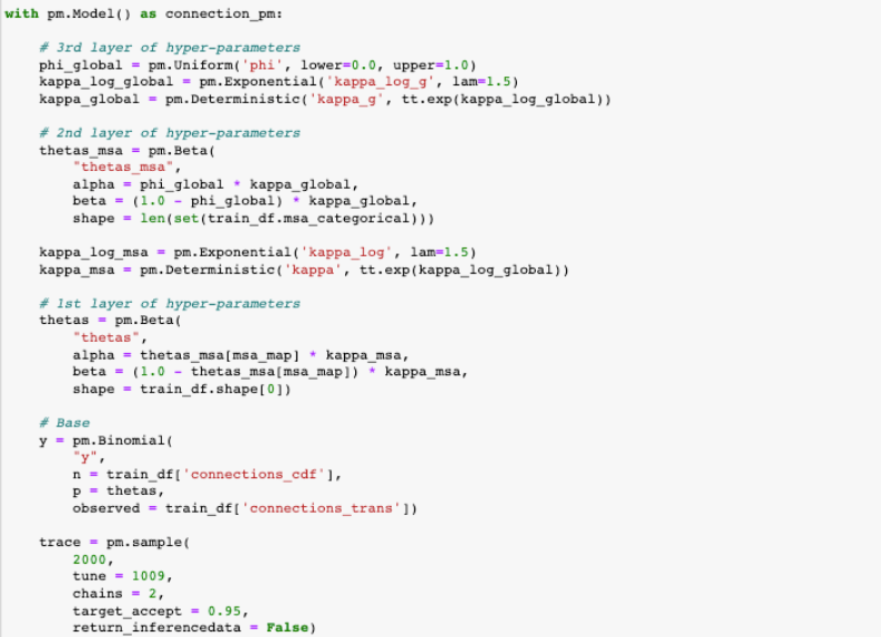
When specifying hierarchical models, the convention is to list the distribution families, parameters and hyper-parameters relevant to each layer of the hierarchy. Extending the above zip-level conversion rate example into a hierarchical model might look like this:

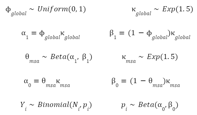
In the above specification, we have re-formulated the Beta distributions parameters into the mean and variance, as described in the PyMc3 documentation.

The Python package PyMC3 solves Bayesian Inference problems without manual calculation. PyMC3 uses Monte Carlo Markov Chain (MCMC) to simulate the posterior distribution and produce as many samples as we like from the posterior distribution. From these samples, you can plot the pdf curve and calculate the mean, median, standard deviation, and quantiles. 

As we specified chains = 2 in the code, we got 2 arrays of MCMC samples as shown below. These two arrays are quite similar, indicating the model has converged and both arrays represent the posterior distribution very well. In our case, we chose the mean of one of the arrays as the zip-level conversion rate.

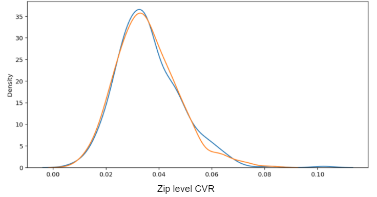
The following plot displays the result in the form of the empirical MSA-level CVRs vs. the modeled, posterior MSA-level CVRs. In this case, we took the mean of the posterior distributions to get a single point estimate for each MSA. 

You can see that the distribution of empirical CVRs 1) is heavily right-skewed and 2) has observations at 0%. Both of these are characteristic of attempting to measure rates for levels with very limited amounts of data. In the posterior CVR, there are no longer 0% estimates and the skewness is greatly reduced. There are more observations at the center of the distribution, reflecting the “shrinkage” towards the mean.

Conclusion

The transaction and engagement team at Zillow Group frequently uses Bayesian methods for our analyses. A separate but very important consideration that has been left out of the above is censoring; unlike a transaction for something like an ecommerce platform, a real estate transaction may take several months to complete. We need to account for this relatively long period of time, during which we may not have observed if the connection will not transact or just has not transacted yet. In practice, the approach described above is augmented to account for censoring.

If you are interested in these topics, consider applying to our team.

References

1. Reich, B. J., & Ghosh, S. K. (2021). Bayesian statistical methods. Chapman & Hall/CRC. 
2. https://www.bayesrulesbook.com/chapter-3.html