In this article we show how we improved the performance of the Zestimate with a de-noising, autoencoder imputation model.

At Zillow we are sitting on a treasure trove of housing data. Our data is collected from multiple sources spanning all regions of the USA. Missing data patterns and representations of home data vary among our data providers, making data reconciliation a challenging process. How do we leverage all of this varied data in order to best predict home values across the country?

Accurate machine learning, including the generation of reliable Zestimates – Zillow’s own ML-generated home valuations – relies on substantial quantities of high-quality data. Original data sources such as ours can nevertheless contain partial omissions. For example, we know a home’s square footage, but lack information on the number of bedrooms. Original data can also contain numerical errors such as a 2000 sq ft home claiming 20 bathrooms. Allowing such inaccuracies to go undetected and overlooked can negatively impact our models and, ultimately, the accuracy of our home valuations. We combine our extensive data with machine learning techniques and domain knowledge in order to impute missing or unlikely feature values that are required by the Zestimate model. Together, this provides our website visitors and internal partners with the best representation of a home’s value.

In this article, we will:

• Describe various statistical and ML tools available for data imputation
• Provide details of different autoencoder methodologies that have proven effective as data imputation solutions
• Describe the data sample used to train and evaluate our imputation models, and discuss our feature engineering techniques
• Compare the performance exhibited by various imputation models on our designated test data sample
• Discuss the impact of our imputation model on the performance of the Zestimate
• Delineate the architecture and design considerations that enable the imputation model pipeline to be integrated into our production workflows

Imputation methods 

Determining which imputation method is optimal depends on the nature of the dataset under consideration, as well as the presence (or absence) of patterns in the corrupted fields. It is not valid to claim one imputation method is better than another universally. One must also consider the downstream application of the imputed data in order to choose suitable metrics to evaluate model performance. 

Various single-value imputation techniques include mean, median, mode and nearest neighbor interpolations (e.g., kNN ); Gaussian kernels; linear quadratic estimations (Kalman, 1960); and least squares polynomial fits (Savitzky et. al 1964). Multiple imputation schemes (MI) (Rubin 1987) generate multiple imputed datasets by imputing missing values repeatedly, such as Multiple imputation using Chained Equations (MICE) (Van Buuren et al.2011).

However, these methods may be unsuited for noisy high-dimensional data with diverse data types, non-linear relationships, and prominent regional missing data patterns – all of which are attributes typical of housing data. Relationships among home attributes such as the square footage, number of bedrooms and number of bathrooms make home attribute imputation via prediction an obvious choice. 

Yet a convoluted interplay exists among home attributes that are generated by latent processes tied to regionally varying and temporally changing homeowner needs. Non-linear interactions among home attributes are frequent within housing data, and uncovering such relationships has proven advantageous for accurate home price evaluations. 

For example, the current Zestimate pipeline captures non-linear feature relationships through a neural network model that outperforms legacy (i.e., non-deep learning based) Zestimate methods (Building the Neural Zestimate). Therefore, we pursue models that are capable of discovering complex nonlinear relationships among high-dimensional data.

Autoencoders are emerging as a popular approach for imputation due to superior performance on diverse datasets (Pereira et al 2020). At Zillow, we explore autoencoders as imputation techniques due to their:     

• Functional flexibility—Denoising autoencoders can be optimized for various use cases, such as imputing outliers or missing data, and they are modifiable to accept fewer – or a greater number – of features.                              
• Robust handling of high dimensional data sets—The absence of distance metrics means autoencoders do not suffer from the curse of dimensionality, and they can exploit the full set of features and their complex interactions.   
• Multivariate imputation—Autoencoders inherently perform imputations across all features with missing values, while simultaneously considering their interdependencies.

Beyond autoencoders, we evaluate kNN, Random Forest, median, and mean imputation methods applied to our data. The following section briefly outlines the mechanisms of a vanilla autoencoder and related variations adopted for this research.

Autoencoders

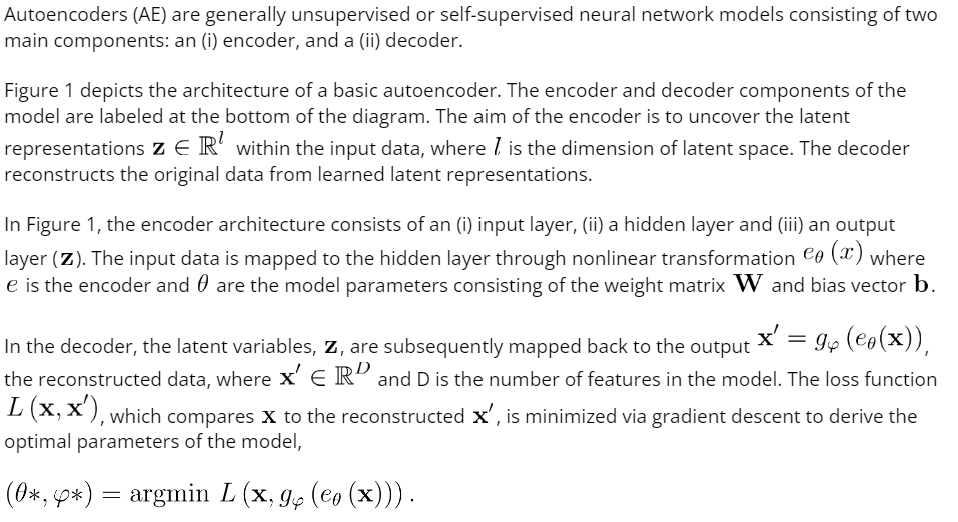
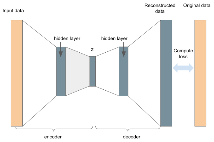Figure 1: A basic autoencoder architecture

Undercomplete autoencoders are a type of autoencoder that transforms input data into lower-dimensional latent space by employing hidden layers with fewer dimensions than the input layer (a bottleneck layer). Analogous to other dimensionality reduction techniques (e.g. PCA), undercomplete autoencoders aim to preserve important structures within the data while discarding noise and superfluous information. 

Conversely, overcomplete autoencoders can be prone to overfitting, which can result in the model learning the identity function – from which we would gain nothing. Dimensionality reduction methods are nevertheless sensitive to noisy and corrupt data which impedes their immediate use as imputation model candidates. To address these challenges, several groups have developed architectural variants of basic autoencoders (see Pereira et al 2020 and references) that are more relevant to ML data preparation at Zillow.                    

Denoising Autoencoders (DAE)

One of these approaches is the Denoising Autoencoder (DAE; Vincent et al. 2008). In this autoencoder variant, input data is corrupted by randomly selecting a proportion of the values to be zero (i.e., a dropout is applied to the input layer)/noise is injected into the input data. The model then learns how to reconstruct the original data  from the corrupted data. Corrupting the input prevents the model from learning the identity function and makes it more robust to overfitting. The DAE is trained to recover missing values and remove noise from the data making it an attractive option for data imputation. In our testing we build our DAE according to the architecture illustrated in Figure 2.

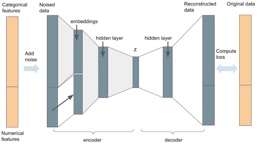Figure 2: Our DAE architecture

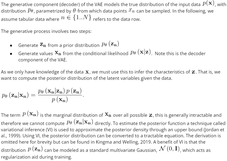
Variational Autoencoders (VAE)

To adapt the autoencoder structure, Kingma and Welling, 2014 proposed an alternative variant of autoencoder, a generative model known as the variational autoencoder (VAE). The VAE still consists of an encoder, and a decoder; however, the encoder and decoder are now probabilistic rather than deterministic.                                           

Latent variables are modeled as distributions rather than points and training is regularized by expanding the loss function to constrain the functional form of the latent space to a standard multivariate Gaussian (or another parameterizable distribution). Modeling the latent variables like this prevents overfitting and ensures a continuous latent space. For more details see Appendix 1.                                        

In practice, the encoder is built as a neural network that ingests the input data and outputs two latent space vectors, one representing the mean and the other the variance of the latent space Gaussian distributions. The decoder is a neural network that samples the latent distributions to form a vector of latent variables z. Back-propagation cannot handle sampled data; therefore sampling must be carried out via the ‘reparameterization trick’ described in Kingma and Welling, 2014. Transforms applied to the latent variables recreate a representation of the original data, as with a standard autoencoder. The encoder and decoder are concatenated to construct the full VAE model. In our testing we build our VAE according to the architecture illustrated in Figure 3.

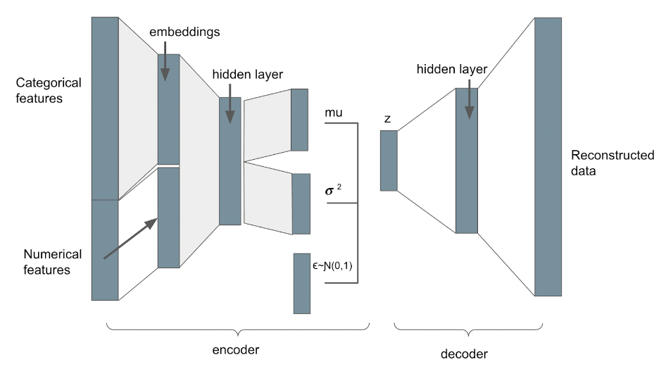Figure 3: Our VAE architecture

Data and feature engineering

Data

Zillow has a total dataset comprising more than 100 million homes, so in order to efficiently iterate through model variations we created a subsample from the complete dataset, specifically drawing from several major Metropolitan Statistical Areas (MSAs). The subsample encompassed 1 million homes for training purposes and 100 thousand homes for scoring.

Feature engineering and transformation

Before constructing the model, we carried out feature engineering as outlined in this section.

Geospatial information, such as Uber’s h3 index and census regions, can be informative predictors of both property attributes and prices. However, this type of data can present challenges due to its high-dimensionality and sparse categorical nature, making traditional one-hot encoding unsuitable. To tackle these issues, we devised numerical surrogate values that consolidate feature information across regional categories, such as quantiles of square footage, or the mode of bedroom counts within a specific geographical region. 

To ensure stability in our neural network models, we used quantile transforms on our numerical variables. This counteracted the potential instability caused by neural networks learning from uncalibrated distributions with varying ranges, as discussed by Krogh et al. in 1991. 

To accommodate mixed input features (both categorical and numerical), we reduced the dimensionality of categorical fields by creating embedding layers for each categorical variable. The categorical embedding layers were combined with the numerical inputs to shape the input layer of our autoencoder models.

Autoencoder models rely on clean data for accurate data reconstruction, so we took steps to mitigate the impact of erroneous data by adopting basic data cleaning techniques, including the removal of outliers identified through domain-specific, knowledge-driven heuristic rules. 

For features with significant missing values, we filled in the gaps using geographical aggregates, and applied a mask to the imputed cells when calculating their loss.

To account for different variable types, we integrated numerical (mean square error) and categorical (cross entropy) loss functions within our autoencoder model.

Comparing imputation model performance

The abovementioned autoencoder techniques have demonstrated strong performance on benchmark image (MNIST) and other low-dimensional tabular data, such as the wine data set. To assess whether these autoencoder methods translate to our use case, we devised a framework that allowed us to evaluate their viability for imputing home attributes within the Zestimate pipeline.

Metrics 

Before testing the impact on the Zestimate values, we needed a way of evaluating the performance of the imputation routine on our data sample.                         

We created a suite of standardized metrics to compare the performances of our imputation models. For initial proof-of-concept, we base these performance metrics on a reduced number of features that we recognize are particularly important indicators of a home’s value (e.g., square footage). There is a strong rationale for evaluating model performance using this reduced set of features: By concentrating on these key features, we take advantage of our domain knowledge of home attributes when constructing our metrics. 

For instance, a 25% error in bedroom count typically has a different effect on price compared to a 25% error in lot size. Similarly, a discrepancy of two years in construction date will impact price differently than a two-unit error in bathroom count. By using a reduced set of features for evaluation, we can create models with a performance that is more interpretable for their downstream use cases within the Zestimate. 

Tailored metrics were created for each of the features of interest. For instance, we considered what percentage of imputed bedroom counts, derived from unseen corrupted data, fell within n units of the original bedroom counts with n being [1, 2, 3]. Similarly, what percentage of imputed square feet are within n units of the original number square feet where n is [100, 200, 500…]; the full set of metrics are shown in Table 1. 

In this manner, we evaluated each imputation model on a feature-by-feature basis, enabling us to optimize decisions based on our prior domain knowledge about the features most relevant for predicting home values.

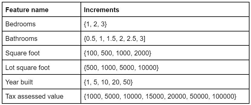Table 1: The full set of increments used to measure the percentage of imputed values that fall within each increment of the true value for each feature.

Model variants

We conducted extensive testing of our models, exploring different model architectures, hyperparameters, and loss functions, both with and without the incorporation of engineered features. Using the metrics defined previously, we assessed the performance of various model families as outlined in Table 2 below. Our models were benchmarked against the baseline of median value imputation, that is, imputation via the median value of a feature.

Across all variations of autoencoder models, we adopted a symmetrical architecture comprising an input layer, a hidden layer, and latent space layer for the encoder, as well as latent space, hidden layer, and output layer for the decoder. The autoencoders were implemented in PyTorch. The denoising AE architecture is depicted above in Figure 2, while the architecture of the variational autoencoder is depicted above in Figure 3.

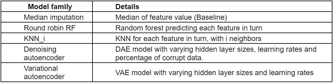Table 2: A description of the imputation model variants tested on sample data.

Imputation model results

We ran multiple iterations of each model and, based on the defined metrics, we selected the best performing from each model category to enable a performance comparison between categories. Figure 4 illustrates the comparative performance of each model in relation to the baseline median approach for imputation of a home’s build year (a), lot size (b), and bedrooms (c). The y-axis quantifies the percentage increase in predictions falling within a certain range (x) of the actual value when contrasted with the median approach. 

As an example, the initial bar on Figure 4(a) (graph on the left) illustrates that the denoising autoencoder outperformed the median by 10% in terms of build year predictions falling within a margin of one year of the actual value.

Figure 4: The comparative performance of each model in relation to the baseline median imputation approach for imputation of (a) build year predictions, (b) lot size square footage predictions, (c) bedroom predictions.

In a qualitative summary of findings:

• For all features,  with the exception of lot size,  every model outperformed the baseline median value imputation approach. 
• With the exception of the denoising autoencoder, all models struggled to predict lot sizes (Figure 4 (b)).
• The random forest model and kNN models showed comparable accuracy to the autoencoder when predicting square footage and number of bathrooms, but fell short when imputing other attributes, such as lot size, bedrooms and build year.
• The variational autoencoder exhibited similar performance to the denoising autoencoder when predicting home tax values, and better performance than the denoising autoencoder when predicting the number of bedrooms, as shown in Figure 4 (c). However, the variational autoencoder struggled to predict other features, such as lot size and number of bathrooms.
• Based on the sampled data, and according to the defined metrics, the denoising autoencoder model consistently performed on par with, or better than, other models,.

Consequently, the denoising autoencoder is the model we have chosen to be developed at scale.

Impact on the Zestimate

Evaluating the Zestimate performance

We evaluate the performance of the Zestimate through a methodology that involves training the model to predict home values from a historical point in time. To prevent any inadvertent data leakage, we ensure that the input data for training is restricted to information available to us prior to the prediction date. Projected home values are mapped to home sale data for sales that occurred within a given window, post the prediction date, to create tuplet ‘sale-pairs’. Thus, the sale-pairs contain the Zestimate predicted value and the actual amount that the home sold for. Using the sale-pairs, we derive standard metrics such as MAPE (Mean Absolute Percentage Error) and MdPE (Median percentage error) over a variety of data segmentations. 

Within this evaluation framework, we compared the performance of our production model with the new model, incorporating imputed data on the sample data set.

Results

In Figure 5 below, the left-hand graph depicts the difference in MAPE between the predictions from the revised code with imputations and those from the production model. A negative value in this context signifies that the predictions from the new model exhibit lower MAPE compared to those of the production model, implying improved model performance. It is noteworthy that the extent of improvement escalates in correlation with the number of imputed features, up until five imputed features. However, beyond this point, while the new version still outperforms the production model, the improvement is not as substantial as that observed for four  imputed features. 

This pattern is logically coherent: with fewer imputations, the imputed data is more similar to the production input data. Conversely, when dealing with a substantial number of missing data fields, the imputation model could encounter challenges in generating accurate imputed values.

On the right-hand side, the graph depicts the difference in magnitude of MdPE between predictions from the two models. For both iterations – production and imputed – the direction of the MdPE of the imputed data is consistent with the direction of the MdPE of the production data (either both positive or both negative). There are minimal and inconsequential increments in magnitude in MdPE for 0-4 imputed features. For the sample with five imputed features, there is a greater reduction in the magnitude of MdPE, but it is a smaller sample and the error bars are large.

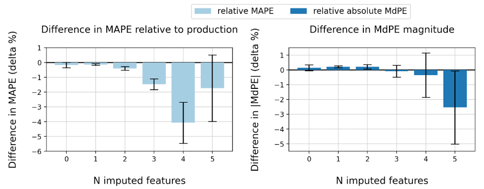Figure 5: The difference in (a) MAPE and (b) relative MdPE between the predictions from the revised code with imputations and those from the production model. The error bars show the 95% confidence interval.

In addition to measuring the performance across the entire data set, we assess the impact of the imputation model on predictions for the subset of homes that lack public record information. Figure 6 shows the results. We see substantial improvements in model performance across all levels of imputed features for both MAPE and MdPE. These particular homes are missing at least one important feature and constitute approximately 5% of our data set.

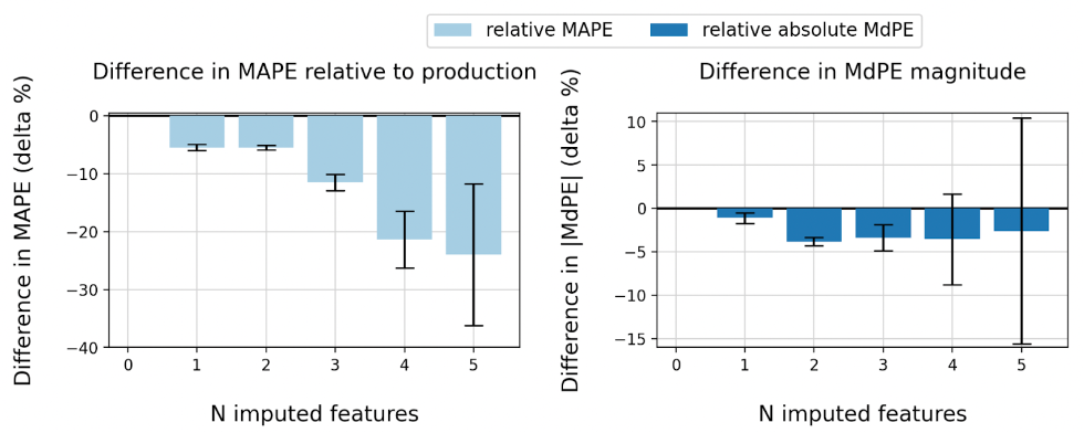Figure 6: The difference in (a) MAPE and relative (b) MdPE between the predictions from the revised code with imputations and those from the production model for homes without public record information. The error bars show the 95% confidence interval.

Building the imputation model at scale

When preparing the large-scale development of our model, we outlined the architecture of the pre-processing, modeling, and post-processing stages to ensure smooth integration into the current Zestimate pipeline.

Our imputation pipeline design was formulated in accordance with the following principles:

• Decoupled training and scoring: A clear separation between the training and scoring aspects (ETLs and modeling) should be enforced, facilitating independent operations.
• Parallel ETL processing: Where feasible, ETL processes should be architected to run in parallel for efficiency.
• Stateless scoring component: The scoring component of the pipeline should be designed to allow stateless processing, enabling the imputation of data for individual homes, one at a time.
• Batch scoring capability: The scoring component of the pipeline should be configured to accommodate batch scoring, allowing parallel processing when needed.
• Consistent data format: At the completion of the pipeline, the imputed data format should mirror that of the non-imputed data to ensure compatibility with existing systems and the flexibility to revert to non-imputed data if required in the future.

Zillow’s AI platform team has empowered researchers by providing a set of tools for efficient and seamless creation and execution of ML workflows. This is achieved via a Workflow SDK, which capitalizes on KFP (Kubeflow Pipelines) to operate on Kubernetes clusters. The WorkFlow SDK is constructed on top of the MetaFlow framework. Metaflow is an open-source Python library that offers a unified API to the entire infrastructure stack. 

As described in the documentation, MetaFlow ‘takes care of the plumbing in an ML pipeline’. The MetaFlow package makes it easy to build pipelines with instinctive DAG (Directed Acyclic Graph) structures. In this context, each node in a DAG corresponds to a ‘step’ in the pipeline. The ‘steps’ function as abstractions, orchestrating the execution of underlying code at each stage. Data exchange between steps is facilitated through the graph’s edges.

We use the WorkFlow tools to build the autoencoder model workflow and the full imputation pipeline (including ETLs and feature engineering). The synergy between the WorkFlow SDK and MetaFlow simplifies resource management for each step and allows for parallelization, or bypassing, of specific pipeline stages. These tools enabled us to align our pipeline design with the principles outlined above.

Closing thoughts

Autoencoders aim to recover latent variables that represent the data-generating mechanism of the observed data. Our preliminary research highlighted that a denoising autoencoder would be a good fit as an imputation model for Zestimate data. Evaluating Zestimate predictions with and without the denoising autoencoder imputations revealed noteworthy improvements in the performance of the Zestimate model, when run on the imputed data. The new imputation model is now in production.

Acknowledgments

A special thanks to Tzu-Hsuan Wei for all his ML engineering work to get the model to production.

References

1. Kalman, R. E. (March 1, 1960). “A New Approach to Linear Filtering and Prediction Problems.” ASME. J. Basic Eng. March 1960; 82(1): 35–45. https://doi.org/10.1115/1.3662552
2. Savitzky, A. and Golay, M. J. E. (1964). Smoothing and Differentiation Of Data By Simplified Least Squares Procedures.. Analytical Chemistry, 8(36), 1627-1639. https://doi.org/10.1021/ac60214a047
3. Toutenburg, H. Rubin, D.B.: Multiple imputation for nonresponse in surveys. Statistical Papers 31, 180 (1990). https://doi.org/10.1007/BF02924688
4. Azur, M.J., Stuart, E.A., Frangakis, C. and Leaf, P.J. (2011), Multiple imputation by chained equations: what is it and how does it work?. Int. J. Methods Psychiatr. Res., 20: 40-49. https://doi.org/10.1002/mpr.329
5. Building the Neural Zestimate – Zillow Tech Hub
6. Pereira, Ricardo Cardoso & Santos, Miriam & Rodrigues, Pedro & Henriques Abreu, Pedro. (2020). Reviewing Autoencoders for Missing Data Imputation: Technical Trends, Applications and Outcomes. Journal of Artificial Intelligence Research. 69. 1255-1285. 10.1613/jair.1.12312. https://doi.org/10.1613/jair.1.12312
7. Pascal Vincent, Hugo Larochelle, Yoshua Bengio, and Pierre-Antoine Manzagol. (2008). Extracting and composing robust features with denoising autoencoders. In Proceedings of the 25th international conference on Machine learning (ICML ’08). Association for Computing Machinery, New York, NY, USA, 1096–1103. https://doi.org/10.1145/1390156.1390294
8. Kingma, D. P. & Welling, M. (2014). Auto-Encoding Variational Bayes. 2nd International Conference on Learning Representations, ICLR 2014, Banff, AB, Canada, April 14-16, 2014, Conference Track Proceedings, .http://arxiv.org/abs/1312.6114
9. https://www.uber.com/blog/h3/
10. Anders Krogh and John A. Hertz. (1991). A simple weight decay can improve generalization. In Proceedings of the 4th International Conference on Neural Information Processing Systems (NIPS’91). Morgan Kaufmann Publishers Inc., San Francisco, CA, USA, 950–957.https://dl.acm.org/doi/10.5555/2986916.2987033
11. MNIST handwritten digit database, Yann LeCun, Corinna Cortes and Chris Burges
12. Wine – UCI Machine Learning Repository
13. https://pytorch.org/
14. What is Metaflow
15. Jordan, M.I., Ghahramani, Z., Jaakkola, T.S. et al. An Introduction to Variational Methods for Graphical Models. Machine Learning 37, 183–233 (1999). https://doi.org/10.1023/A:1007665907178
16. Kingma, D.P. and Welling, M., 2019. An introduction to variational autoencoders. Foundations and Trends® in Machine Learning, 12(4), pp.307-392. https://arxiv.org/abs/1906.02691

Appendix 1