Optimizing Elasticsearch for Low Latency, Real-Time Recommendations
At Zillow, we incorporate personalized recommendations in many product areas to improve the user experience. The recommendations are incorporated into search results, Home Detail Page recommendation modules, and personalized collections, such as on the mobile updates tab.
These APIs must be low latency so that page load time is not impacted. Previously, we relied heavily on batch systems to provide recommendations for experiences other than personalized search results. This year, we have focused on generating most of our recommendations in real-time. Generating recommendations in real time allows us to capture new listings that come on the market and the most up-to-date user preferences.
The architecture behind real-time recommendations
First, let’s take a look at the architecture of our real-time recommendation system. We use a combination of Java and Python for our services, Redis for distributed cache, Elasticsearch for candidate generation, and streaming data architecture for real-time updates to listings and user profiles (not included in the architecture below). We selected Elasticsearch as our listing back end because we require the ability to perform custom relevance sorting for each request.
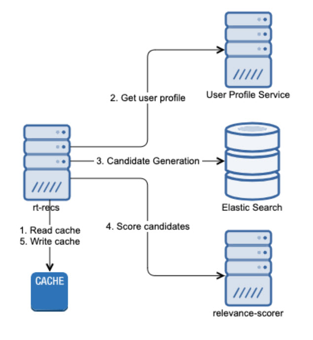

When a request comes into the real-time recommendation service (rt-recs), the following happens:
- Check Cache: The Redis cache is checked to see if a cached request can be returned.
- Get User Profile: The user profile is requested from the User Profile Service. The user profile is updated in near real-time to reflect the user’s preferences.
- Candidate Generation: The user profile, request arguments (filters such as location, min/max price, etc.), and configuration parameters are used to generate an elastic search request for candidate generation. The relevance score for the document is based on a linear model generated from the user profile. Elasticsearch must generate a maximum of 100 candidates from approximately 1.3 million listings.
- Score Candidates: The relevance scorer is a Python service that scores the candidates and typically returns less than 10 recommendations.
- Write to Cache: The response is cached, if applicable.
Each stage above is associated with a Hystrix circuit breaker timeout to ensure the request can be completed within the service-level agreement. The request spends the largest proportion of its time in the candidate generation phase. Historically, this has been the source of bottlenecks and timeouts for our real-time recommendation service.
The life span of an Elasticsearch request
An Elasticsearch request consists of three main phases: queue, query, and fetch. If all search threads are busy when the request reaches Elasticsearch, the request will wait in the queue.
Consistent large queue lengths or thread pool rejections indicate a capacity issue. Document IDs matching the query parameters and scoring are generated in the query phase. The document content associated with each document ID is fetched in the fetch phase. In addition to these three phases, network latency between the calling service and the Elasticsearch cluster is dependent on location and payload size.


To understand how much time the request is spent in each phase, we run the following:
GET /_stats/search
The results show the aggregated time and request count since the cluster was last restarted. The “query_time_in_millis/query_total and fetch_time_in_millis/fetch_total” command can be used to determine the average time spent in each phase.
Our cluster had a 40%–60% split between the average time spent in the query and fetch phases. This indicated that we could likely optimize the time spent in the fetch phase. On the other hand, a significant amount of time spent in the fetch phase is usually an indication of slow disks, document enrichment (not applicable in our scenario), or requesting many or large documents.
Fetch Methods in Elasticsearch
Elasticsearch uses three types of fetch methods: source, stored field, and doc values.
The source field is the original JSON document sent to Elasticsearch when the document is indexed. The source field is the first stored field in the row corresponding to that document ID. Source filtering can be applied by querying using the “fields” parameter. The entire source will be read and then filtered down to the specified fields. This is the default method in Elasticsearch.
Stored fields are stored on-disk in rows corresponding to the document ID. The source field, if enabled, is the first stored field. To access a stored field, the row needs to be accessed, and fields before the field of interest need to be skipped by length.
Doc values are stored in an on-disk, column structure. The field value of each document is stored consecutively in memory. This makes accessing a certain field for a given document straightforward, without loading or skipping other fields. Doc values are stored for supported fields by default (text and text-annotated fields are not supported).
The decision of which fetch method depends on which types of fields you need to query, which methods support them, and how many of the fields in the source must be returned. Fetching the source field will be most efficient if the entire source needs to be returned. If only a small number of the fields included in the source need to be returned, doc values will be the most efficient. Stored fields will not be the most efficient at either end, but is a tradeoff between the two approaches.
We switched our fetch method from source to doc values in production and saw considerable performance improvements. Not only did the fetch time decrease, but the decreased payloads also improved network latency and computation expenses of JSON load/parse in rt-recs and relevance scorer.
The change decreased rt-recs CPU by 38.7%, Elasticsearch dropouts by 54.7%, relevance scorer dropouts by 44.1%, and total dropouts by 2.5% in production. Overall service latency decreased by 11.5%, 14.6%, 22.2% and 25.6% at the 50th, 75th, 95th and 99th percentiles, respectively.
The reduced payload size resulted in a forecasted sizable AWS data transfer cost savings.

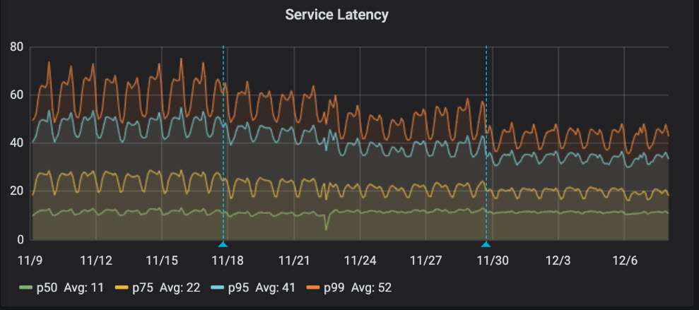
Overall service latency prior to rollout (first third), during the 50% A/B test (middle third), and at full rollout (final third)
Caching in Elasticsearch
Elasticsearch utilizes three types of caches: the page cache, request cache and query cache.
The page cache (or filesystem cache) happens at an operating system level. It will place data read from disk into memory so that the next time that data is accessed, it can be read from memory. Elasticsearch relies heavily on the filesystem cache, which is why it is recommended to reserve at least half of the system memory for the filesystem cache.
The request cache is per shard and caches full responses to requests. Since we utilize Redis to cache full responses from the entire system, it does not make sense for our application to use the request cache.
The final type of cache, the query cache, is enabled by default and uses 10% of heap memory. The query cache will cache individual parts of a query by creating a bitset for which documents match the query. For example, if a query contained a common price range searched for, Elasticsearch may choose to cache the results of this part of the query, even if the rest of the query contained other filters.
The way the Zillow UI is defined helps us have cacheable queries for some commonly searched ranges such as price or square feet, since the UI has suggested values or dropdown menus. Our cluster has an average 63% cache hit rate. The query cache statistics can be viewed by running the following:
GET /_stats/query_cache?human
The tradeoff between consistency and performance
As with any database, a tradeoff between indexing performance and search performance must be made in Elasticsearch. In our scenario, it is more important to be able to provide very low latency home recommendations with the risk that some of those recommendations could be based on slightly stale data (such as if a listing price has been updated).
Bulk requests
Updates to our Elasticsearch come via streaming architecture, and can be either data updates (such as a new listing or updated price) or updates from other pipelines we use to enhance data such as adding home insights, popularity score or a prediction of how quickly the home will sell.
We rate limit these updates to Elasticsearch and use the bulk processor to send batches of updates to Elasticsearch. Trying to use too large of a bulk size will put the cluster under memory pressure. We determined the optimal bulk size empirically by running a series of load tests under realistic load conditions and varying the bulk size.
Refresh Interval
The refresh interval determines how quickly a document will be available to search after it is indexed. When the refresh happens, all the changes in the memory buffer since the last refresh are written to a new segment.
The default refresh interval in Elasticsearch is 1s. When the refresh happens, the query cache becomes invalid. Since our application does not critically depend on the data being available as soon as possible, we have increased this setting to take advantage of having a longer lived query cache.
Conclusion
Overall, we were able to adapt Elasticsearch to provide low latency search with customized relevance scoring. Through a series of load tests, we were able to determine optimal settings for our cluster. We experimented with fetch type, caching strategies and indexing settings to achieve the low latency required to provide real-time recommendations to users on Zillow.