Perhaps not surprisingly, one of the most important features for home recommendations is a user’s location.  In this blog post, we first discuss a simple baseline method for modeling a user’s location preference based on zip-code counting. In the second part, we outline an alternative method based on clustering past user home clicks and building a personalized click density model for each individual user.

Home Recommendations

The Personalization & Relevance team within Zillow’s Artificial Intelligence group (formally known as Data Science and Engineering) is responsible for developing a personalization layer across various products such as search and email. The main mission of our team is to make it easier for Zillow’s users to discover and find relevant home information and we strive to guide users through all aspects of the real estate market. We learn from a user’s interaction history on the website and in the mobile apps and then customize the displayed content accordingly.

One of the core products developed by our team is a content-based home recommendation engine. The engine builds a user profile for each user and upon request makes recommendations by 1) generating a set of candidate homes and 2) ranking these homes based on a predicted match between the user profile and the candidate homes. This prediction is based on various features. Below we discuss two ways to construct input features capturing user’s location preference.

Zip-code counting

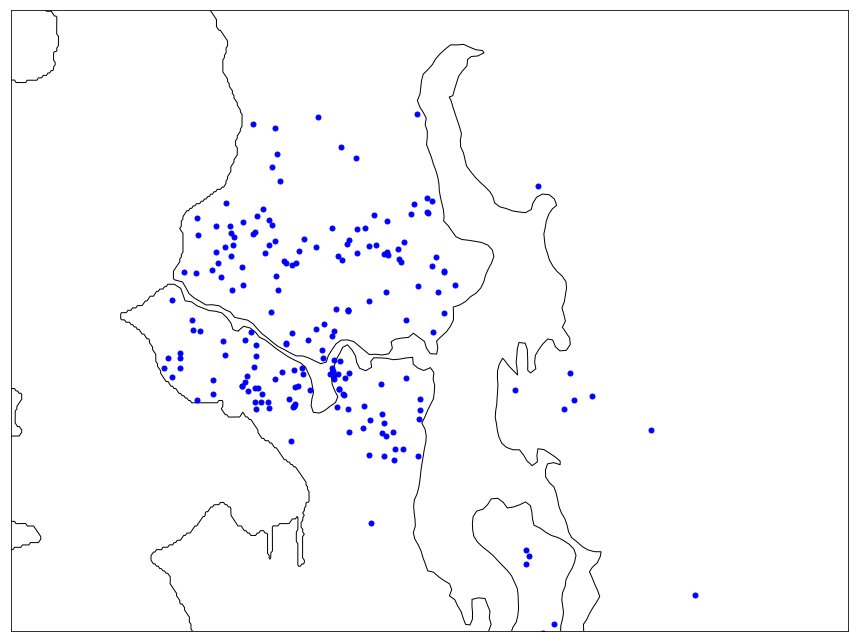
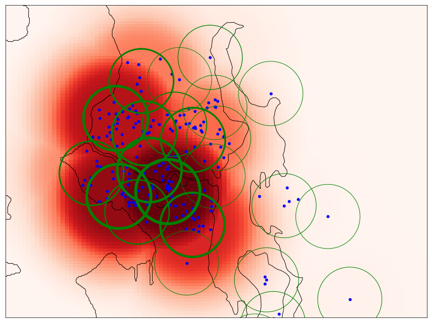
According to the Zillow Consumer Housing Trends Report, the typical US home buyer spends 4.3 months searching for their new home. During this time, users repeatedly visit our site and apps, search their target area, and interact with listed homes. This interaction history can be viewed as a random sample from some unknown location preference density function. We can assume that areas in which  users explored more homes are more likely to be relevant to that user. Furthermore, for near-future home click prediction, areas explored more recently by the user are also more likely to be more relevant . As an example, here is a plot of the locations of the 200 most recently clicked homes by a potential home buyer in Seattle, WA.

Zip-code Histogram

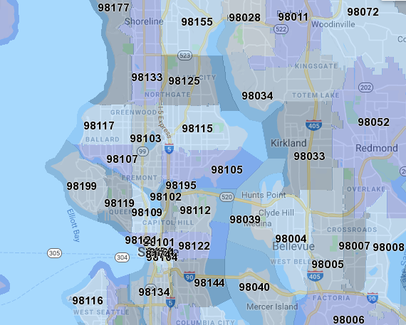
In order to build a user’s location preference profile, we need some way to aggregate and summarize the recorded home interaction history. One intuitive way to do this is to leverage the already existing decomposition of the United States into zip-code areas. The figure below shows the zip-code area subdivision in and around Seattle.

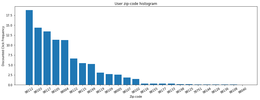
To model the user’s location preference with respect to zip-codes, we can simply count home clicks in each zip-code. To accommodate for time-shifting user preference, we can weight each click with an exponentially decay based on how long ago a particular home was clicked. After doing this, we obtain a user zip-code histogram based on the discounted click frequency as shown below, with the most recent and frequent user home interactions in zip-codes 98112, 98103 and 98117.

Zip-code Location Preference

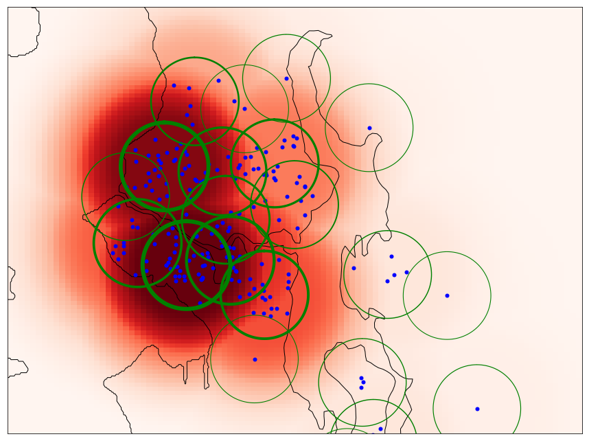
Once this user profile is constructed we can use it to extract features for our user home match score prediction model. For example, we can extract features based on the normalized zip-code histogram count for each candidate home. In our example, homes in 98112 would have the highest value, followed by homes in 98103, 98117 and so on. This method is intuitive, simple to implement and easy to incrementally update as new home interactions are added to the profile. However, it suffers from several drawbacks, especially when it comes to how accurately it models the user’s location preference. To visually understand what this zip-code count based matching feature looks like, we have rendered a map of the zip-code histogram-based location preference. The shade of the color of each cell in the map overlay is assigned based on the nearest zip-codes normalized discounted histogram value (i.e. the darker the shade of red, the higher the location preference value).

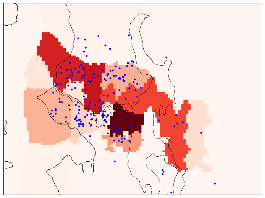
We can see that this location relevance feature is rather discontinuous and does not exactly match our real world intuition. For instance, it is quite likely that two homes very close to each other in terms of walking or driving distance might get vastly different feature values just because they are located on different sides of a zip code boundary. Furthermore, while there are certain aspects of zip-codes that might guide users in their search (e.g., school assignment, or state boundary), most users are likely not aware of the precise zip code boundary, and each user might understand neighborhoods and nearby areas in their own unique way.

Personalized Location Preference

To address the above identified issues, we decided to experiment with a new solution for modeling user location preference that would match our set of desired properties:

• Simple to implement
• Fast, requiring preferably a single pass through the data
• Supports incremental updates as new clicks arrive
• Better predicts the user’s location preference

Intuitively, we first need a way to model the spatial distribution of user clicks, which could then be used to predict future home clicks. To do this we have decided to first cluster the set of user clicks. The reasons for this are both computational since clustering reduces the number of parameters for users with a large amount of clicks, as well as accuracy-related since clustering also reduces noise in sparse data by grouping data points together. However, while there are many available clustering methods to group points in 2D space, not many of them fit our specific needs.

Single Pass Clustering

The Single Pass clustering method fits our needs very well. Despite a lack of any guarantees to produce an optimal clustering, it works just fine for our use case, producing a reasonable representation of a user’s location preference with small computational effort. The pseudocode of the method can be summarized as follows:

• Randomly select a data point, and assign it to a new cluster
• For each remaining data point:
  • Compute the distance to the nearest cluster
  • If the distance is more than max_radius, create a new cluster
  • Else update the nearest cluster by shifting its center towards the new point
    • (The amount of shift depends on the weight of the new data point and the total weight of points already assigned to the cluster)

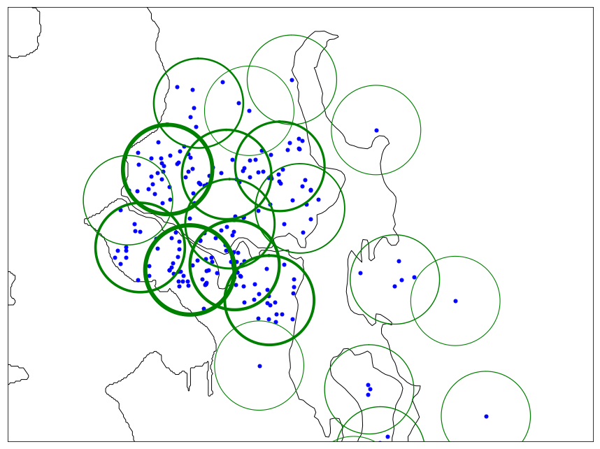
We can see that this method does not require a pre-specified number of clusters, but instead it relies on a maximum cluster radius threshold. We can easily set this threshold based on the preferred location resolution (or even set it dynamically based on home density in a particular area). To show how this clustering works, we have depicted the learned cluster distribution for the sample Seattle home buyer with a maximum cluster radius of 2.5 km. Note, that the width of each cluster’s border denotes its weight. In this clustering, we set the weight of each point to 1; i.e., there is no time-decaying weight.

Cluster Membership Function

Once we construct the user’s cluster-based location preference representation, we can use it to compute the location matching feature between the user’s profile and a new actively listed home. While there are many ways to do this, we have selected a simple method that models the match between cluster and point by using an s-shaped membership function. The nice property of this function is that its parameters are easy to interpret and tune for a specific application. The general definition of the membership function is given be the following equation:

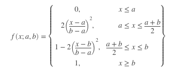
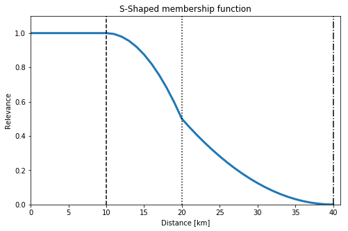
For our purpose, we have adapted the above equation to be decreasing function of the distance and to use cluster radius as parameters; in particular, first-outer radius and second-outer radius. The s-shaped function takes on the value of 1.0 for distances less than the cluster radius, it smoothly interpolates between 1.0 and 0.5 for distances between the cluster radius and the first-outer radius, and finally it smoothly interpolates between 0.5 and 0.0 for distances between the first-outer radius and second-outer radius. As an example, the plot below shows the s-shaped membership function with cluster radius of 10km, first-outer radius of 20km and second-outer radius of 40km.

In order to account for the weight of each cluster, we scale the amplitude of each cluster’s membership function by the cluster’s own normalized weight.  As a result, the cluster with the highest accumulated weight has maximum membership of 1.0, and other clusters have maximum membership proportionally smaller. Finally, for each candidate home, we compute the location match feature as the maximum over the scaled s-shaped membership function with respect to all clusters.

To visually demonstrates what this feature looks like, we have again rendered its value in the Seattle area for the same example user. We can clearly see how the higher values of location preference center around higher-weight clusters, and the overall location relevance function is more smooth and continuous.

Adding time-weighting

Finally, similarly to using exponential decay during zip-code counting to accommodate for recency, we can also incorporate recency into our new cluster-based representation. The Single Pass clustering method can weight each cluster point by its relative importance. All we need to do is to set the point importance based on the exponential decay of how long ago each home was clicked.

To show the effect of adding time-weighting, we render the location match feature value with time-weighted home clicks below. After accounting for time, the user’s location relevance heat-spot moved further to the east close to the South Lake Union area.

Evaluation of Location Preference Features

In addition to visual inspection, we also would like to quantitatively evaluate the contribution of the cluster-based location preference feature. To do this we use a user’s past interaction history and measure how well we are able to predict their home clicks on the following day. We collect all candidate homes, namely the set of homes in the general area where the user is searching, as a search result set. We label homes clicked by the user as positive examples and the rest as negative. Once our content-based recommender engine predicts the user-home match score, we sort all results by this score.

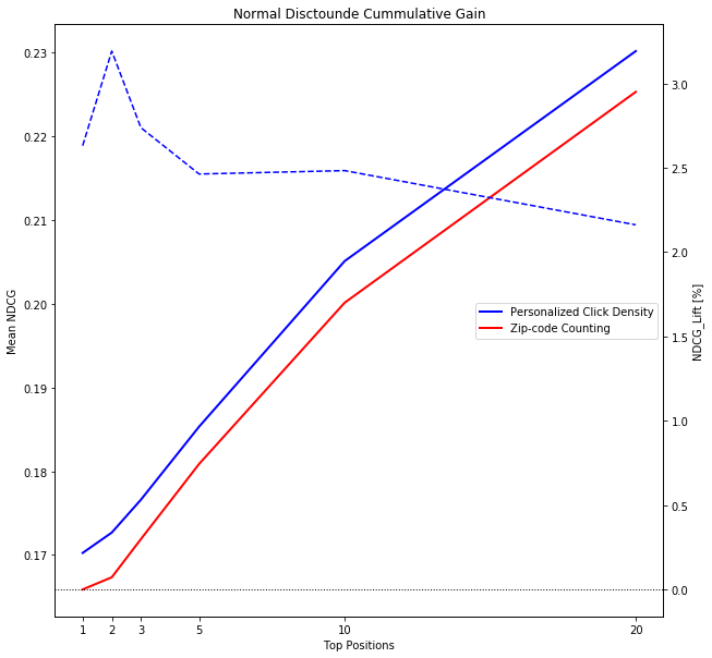
To evaluate the quality of the sort order, we compute the Normal Discounted Cumulative Gain (NDCG). By calculating the relative lift of the mean NDCG between two match score prediction methods, we can gain an understanding of which method is likely to display more relevant homes higher in the sort order. The intuition is that the higher we sort relevant homes, the more likely the user is to view them and engage with the search result set.

The chart below shows the absolute mean NDCG @ 1, 2, 3, 5, 10 and 20 top positions. In addition, the right-hand axis shows the relative lift of the mean NDCG between the user home match score prediction with personalized click density (the blue solid line) and zip-code counting (in red). The plot shows that personalized location preference density can better predict user’s future home clicks than zip-code counting, which leads to an NDCG lift of 3% in the top of the sort and over 2% in the top 20 positions. As a next step, we will be validating the features in production via a live A/B test on the site.

Room for Improvement

In this post we demonstrated that the personalized click density-based location preference more accurately models user behavior. However, there is certainly a lot to be improved. From the heat maps shown above, we can see how our radiating location preference extends across lakes. Perhaps clustering in driving distance space would yield more accurate and intuitive results. Also, our current method uses a single distance threshold value for Single Pass clustering. Clearly, using a dynamic radius based on local listing density should yield additional improvements, i.e. smaller clusters in urban and larger clusters in rural areas.

If you find this work interesting and if you like to apply you data science and machine learning skills to our large-scale, rich and continuously evolving real-estate data set, please reach out – we are hiring.