Clickstream data is one of the largest and most important datasets within Zillow. The data set contains a log of a series of page requests, actions, user clicks and other web activity from the millions of home shoppers and sellers visiting Zillow sites every month. The data powers many reporting dashboards and helps us answer complex business questions. From product initiatives to analyzing user behavior, personalization, recommendations and machine learning all depend on this valuable dataset to generate actionable insights.

We’ve always been successful at collecting this data through a pipeline, but due to the sheer size of the data set, making this ETL process efficient and scalable has been a huge area of focus for the team. With close to a billion events per day received via click stream data, we couldn’t initially scale fast enough to meet the growth in data volumes using our existing system. We sought a distributed platform which would enable the fast parsing and processing of large datasets via a massively parallel processing framework. Ensuring we get this data to the right dashboards in a timely manner is crucial as internal stakeholders are counting on it to make decisions. Our process has gone through several enhancements over time and here’s how we built it:

History

Version 1

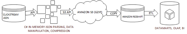
We receive a large batch of raw web activity data in JSON format. On our end, we decided to use Amazon Redshift as our data warehouse and query platform due to its cost-effectiveness and inherent columnar database benefits. Our ETL process involved:

1. Download the JSONs to local.
2. Using C# .NET, parse and convert the JSONs to CSVs while performing a number of transformations along the way. Such as flattening various nested elements, deriving calculated columns, cleaning up text and formatting. We also split the CSV into multiple parts and compress them to make COPY more efficient.
3. Upload CSVs to Amazon S3.
4. Run COPY command in Redshift to copy CSVs from S3 to a Redshift table.

Scheduler: SSIS package via SQL Server Agent.

Version 2

At this point in our company’s growth, the process started becoming slow due to increase in data volume. To make it fast again, we merged steps 1, 2, 3 above into a single step and added multithreading. Here is what it looked like:

1. Read JSON lines into memory, skipping the download. Perform the transformations on the fly using .NET’s multithreading capabilities. Write split CSVs into S3. Based on our server hardware, best performance was noticed when there are 8 parallel threads.
2. Run COPY command in Redshift to copy CSVs from S3 to a Redshift table.

Scheduler: SSIS package via SQL Server Agent.

Version 3

Apache Hadoop is introduced into the picture. MapReduce written in Java. To replace an outdated .NET multi-threaded design. Hadoop cluster is launched and shut down for every run using command line (CLI) tools.

1. Read JSON lines into memory, skipping the download. Perform the transformations on the fly using Hadoop, while writing CSVs into S3 in parallel.
2. Run COPY command in Redshift to copy CSVs from S3 to a Redshift table.

Scheduler: Powershell+SQL Server based scheduling framework. Command line utilities for Hadoop cluster management.

Hadoop Cluster: 100 nodes with 16 vCPUs, 60 GB memory each.

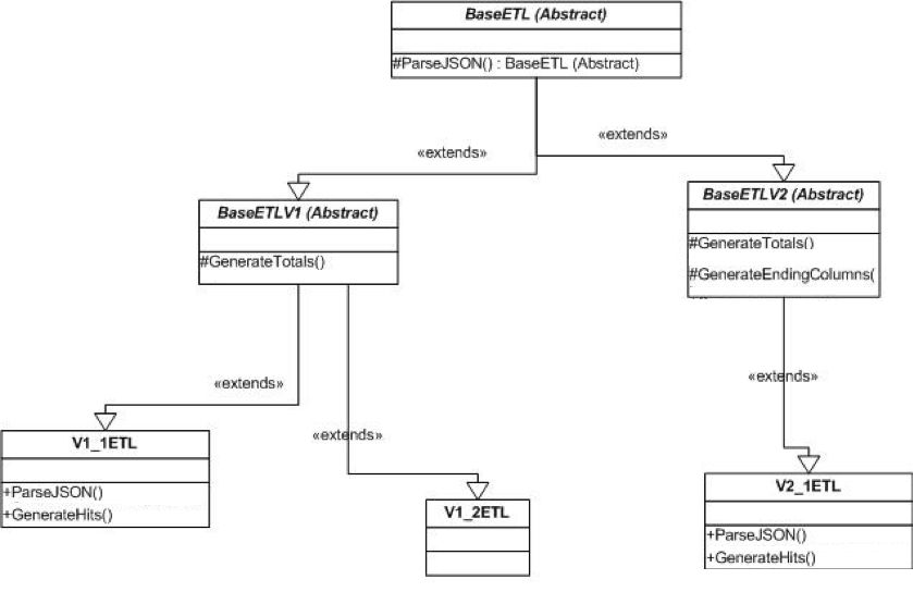
Hadoop MapReduce is implemented in Java. The java code is written such that it can support multiple current and future versions of the ETL and yet require as little change to the code as possible.  This is done via a series of Abstract classes. All versions of the ETL start at BaseETL. From there, Version 1, 2 etc are created. These again are Abstract. Any changes made to BaseETLV2 will show up in any version that extends this. This allows us to make a general fix to all version 2s or all version 1s. The “V” is the actual implementation. This has a ParseJSON function that is called when parsing data. With this Factory Producer based implementation, we need not create instances of any ETL and we instead use the Factory Producer class, which returns the correct version of the ETL we want.

Today

Version 4

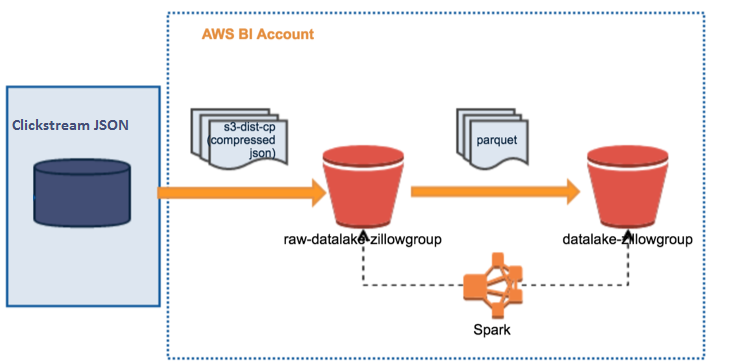
Our web activity data is a collection of events generated from Zillow Group web platforms and mobile apps. Each web platform or mobile app maps to a separate data set in the source system storing the logs each day. For example, zillow.com, Zillow iOS app, Zillow Android app all have their own unique dataset IDs and corresponding source tables, identified using a dataset ID and Date. Dataset IDs are unique IDs for each app. This data is extracted from source table to Zillow Group Data Lake daily for all datasets.

We set ourselves an audacious goal of building a new pipeline that makes the data available in the Data Lake in parquet format after its arrival in the source within 30 minutes. The biggest dataset is about 2 TB uncompressed for a single day. In addition to speed, there were other important decisions such as retries, alerting, auditing to be included in the design to make pipeline reliable. We tried different approaches to get this data in data lake. We decided to go with the one that is not only faster and simpler but can also be modularized in separate tasks. We did this in Apache Airflow, which is now our primary choice of ETL scheduler. One of the main advantages with this approach is the ability to retry from a failed step as opposed to re-running the entire pipeline. For more info on how we use Airflow, refer to an earlier blog post: https://www.zillow.com/data-science/airflow-at-zillow/

As soon as data is available in the source, we issue an export into JSON format. We use a dedicated Amazon EMR cluster for all the processing. The raw data in JSON format is moved over to “zillow group raw data lake” S3 bucket in Zillow Data Lake using “s3-dist-cp”. A Spark job on EMR transforms raw data into Parquet and places the result into “zillow group data lake” S3 bucket.

This latest version of our pipeline is our biggest leap forward and introduces several new big data frameworks in the picture:

• Spark is introduced to replace Hadoop.
• Elastic MapReduce (EMR) cluster replaces a Hadoop cluster.
• Apache Airflow replaces the Powershell + SQL Server based scheduling.
• Hive tables based on columnar Parquet formatted files replace columnar Redshift tables.
• S3 based Data Lake replaces Redshift based Data Warehouse.

1. Copy JSONs to Amazon S3.
2. Run our Spark processing on EMR to perform transformations and convert to Parquet.

Scheduler: Apache Airflow

EMR cluster configuration: A fully scaled up cluster looks like below:

• Master: 1 m4.4xlarge (32 vCore, 64 GiB memory, EBS only storage, EBS Storage: 200 GiB)
• Core: 10 r3.4xlarge (32 vCore, 122 GiB memory, 320 SSD GB storage, EBS Storage: none)
• Task 1: 10 m4.16xlarge (128 vCore, 256 GiB memory, EBS only storage, EBS Storage: 200 GiB)
• Task 2: 15 r4.4xlarge (16 vCore, 122 GiB memory, EBS only storage, EBS Storage: 200 GiB)
• Task 3: 10 r3.8xlarge (64 vCore, 244 GiB memory, 640 SSD GB storage, EBS Storage: none)

Design

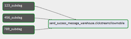
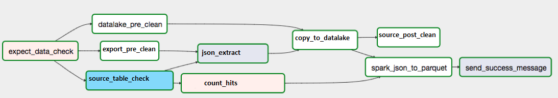
Airflow DAG: DAG is designed to run each dataset independently based on availability of dataset in the source. This is accomplished using SubDags for each dataset. These SubDags are independent and can potentially run in parallel. But we observed issues with race conditions in subdag concurrency and moreover, we did not want to go too crazy with cluster size. So we decided to run the pipeline in a more controlled fashion. We only allow dag concurrency of 1 which means airflow will schedule only one dag run at a time and subdag concurrency of 4 which means 4 datasets can run at a time. In addition to that, we don’t allow two big datasets to run at same time mainly to avoid big datasets competing for resources. This is achieved by using separate pool config in the Airflow with an available slot of 1.

Dag consists of 2 tasks: SubDag task and SNS task. There is exactly one SubDag task per dataset. In some cases, we have a single hive table storing multiple datasets. In such cases, we configure single SNS task dependent on multiple datasets.

SubDag handles everything starting from data availability check to parquet processing.

Example Spark command:

Spark-submit
--master yarn --deploy-mode cluster \
--name Web-Activity-ETL-987654321-2017-10-01 \
--executor-memory 20G \
--driver-memory 5G \
--conf spark.sql.files.maxPartitionBytes=16777216 \
--conf spark.sql.shuffle.partitions=5000 ./weblog/weblog-spark-etl-deploy-bundle.jar \
--data-date 2017-10-01 \
--dataset-id 123456789 \
--role arn:aws:iam::12345:role/web-activity-role \
--src s3://<zillow group raw datalake>/zillow/web-activity/json/ \
--dest /tmp/webactivityspark/parquet \
--num-files 500

Performance: Running spark job for our biggest dataset under 30 mins was a goal. A couple of things that helped in increasing the performance significantly are: (1) Switching from Python to Scala made UDF’s significantly faster as Scala can directly run on JVM. (2) Avoiding ‘explode’ function to extract dimensions in raw data and then join back to original dataset removed extra shuffle cost and caching. Instead of ‘explode’, we use index for each dimension to add new columns as look up happens in constant time.

Configuration: Various components of the entire pipeline are configurable through a YAML config file. A configuration-driven design allows for easy modification of following: (1) Add or remove a dataset ID in our pipeline (2) Update Spark settings for a dataset: spark_opts – It allows spark conf settings along with application args such as driver-memory, executor-memory and output number of files. (3) Update Dag and Subdag parallelism.

Alerting is done via Amazon SNS (Simple Notification Service).

Scheduling: We made sure no two big datasets run at same time on the cluster. This was mainly done to avoid over utilization of resources on Spark cluster. We created a separate pool in the airflow with single slot. We assign this pool for both of these datasets so at any given time if these datasets are picked by scheduler it would run one or the other, but not both. We have subdag concurrency of 4 which means 4 datasets can run at same time.

Hive tables: We store all of the raw web activity data under one primary hive table. Based on the expected query patterns, we chose to partition this parquet-based table on the fields dataset ID and data date. We also have set of secondary tables that are analysts facing and that sit on the same location as above table with exact same table definition. These additional tables are pre-filtered by dataset and provide a similar interface to queries written originally against Redshift.

Hive Metastore: We use Amazon Relational Database Service (RDS) for Hive Metastore. A persistent Hive Metastore removes the need to recreate Hive metadata (e.g. table structures and partitions) each time a new hadoop/spark cluster is started. Additionally, it allows teams across our organization to share the Hive metadata.

Benefits of using AWS

To solve the scalability and performance problems faced by our existing ETL pipeline, we chose to run Apache Spark on Amazon Elastic MapReduce (EMR). By running Spark on Amazon Elastic MapReduce (EMR), we can quickly create scalable Spark clusters and use Spark’s distributed-processing capabilities to process large data sets, parse them and perform complex calculations. Spark on Amazon EMR also meant we did not have to manage the Spark clusters ourselves.

As data volume continues to increase, the choice of Spark on Amazon EMR combined with Amazon S3 allows us to support a fast-growing ETL pipeline: (1) Scalable Storage: With Amazon S3 as our data lake, we can put current and historical raw data as well as transformed data that support various reports and applications, all in one place. So we now have a central place to enable infinite storage scalability at a low cost. All the raw data containing clickstream/user-traffic events is ingested and pushed into Spark on Amazon EMR. From the data lake, a number of applications such as personalization, recommendations, advertising optimization use the data without storage scalability concerns. Web activity is just part of several petabytes of data maintained in our Amazon S3 Data Lake. (2) Scalable Compute: With Spark combined with several features of Elastic MapReduce (EMR), we are able to scale up (or down) storage, compute & memory capacity automatically as well as on demand.

We wished to minimize our costs involved in running the EMR cluster for the duration of the pipeline. Various clickstream datasets processed by our pipeline varied quite a bit in terms of their size i.e. the volume of data and the number of records. This meant that the amount of required cluster resources such as CPU and memory also varied. We could potentially launch an EMR cluster big enough to handle our largest dataset. But smaller datasets which require significantly less powerful of a cluster would make this approach less cost effective. That’s where EMR Auto Scaling comes in handy. For more info on how we use auto scaling, refer to our earlier blog post: https://www.zillow.com/data-science/save-money-emr-autoscaling-spot/

Summary

The ETL job now takes around 30 minutes instead of several hours. Now we get data in the hands of users sooner than before during normal business hours. Due to the increased speed and reliability of our pipeline, clickstream/web activity data is made up-to-date sooner which makes dependent reports and models more accurate because they’re built with the absolute latest data. This is a huge benefit for business stakeholders and users, who depend on this information to influence their decisions.

We process several TBs of data per day and over a billion records per day across our Airflow pipelines. The biggest dataset in our web activity pipeline alone is about 2 TB of data (uncompressed) per day. Our table supporting the web activity data is the widest of our tables with about 700 columns. Due to existing dependent reports and a significantly sized user base already for Redshift, we are currently maintaining both our Redshift based Data Warehouse as well as S3 based Data Lake. Having both these solutions in place allows for a smooth transition from older to newer platforms, with minimal downtime in serving data for end-user’s needs.