SpectroBrain: Detecting Phone Spam with Semi-Supervised Learning

At Zillow Rentals, we cherish the trust and safety of our users with the utmost priority. While renters seeking their next dream home are communicating with property owners/managers using our platform’s email and phone messaging features, spammers also are interested in these same communication channels. For example, spammers have called our users to pitch tax debt relief services or cryptocurrency investments. We must proactively identify and block these unwanted callers.
Zillow Rentals has developed many sophisticated tools to detect and fend off spammers. One such tool uses machine learning to detect spam in voice message recordings, in order to identify the offending callers. In this article, we will explain the application of data-efficient, semi-supervised learning in developing a phone spam detection system known as the SpectroBrain.
The biggest challenge with solving this problem is the lack of labeled training data due to the lack of a direct mechanism for telephone users to report spam to the platform. Our limited analysis shows that a small fraction of answered calls fit into this bucket. Stratifying our sampling approach could increase the observed amount and proportion of spam phone calls in our dataset, but it would still take considerable time and effort to collect and label a large set of examples of spam calls with which to train our models.
Starting with no labeled samples, we collected 530 phone messages (via stratified sampling) and manually labeled them to uncover 48 spam phone calls. We split this dataset into three subsets: 417 for training, 59 for validation, and 54 for testing. As these numbers show, our training set is very small—particularly when considering the massive amount of data that is typically used to train modern machine learning models.
In previous efforts, we have already developed a text-based classifier to detect spam in email communication. A natural first step in spam phone call detection is to leverage this work by automatically transcribing the full voice messages to text and then classifying these transcriptions using the text-based detector. Initially, our tests showed that such a setup results in about 50% false negative rates. Can we improve the prediction performance? Spoiler alert: We can!
Most phone calls today are not answered immediately. Instead, callers are often directed in recorded prompts to leave voicemails. When contacting businesses, callers are also likely to encounter phone menus containing multiple steps and choices before reaching a human operator. Our analysis shows that as many as 80% of phone calls through our platform begin with preambles such as voice-mail introductions or automated menus. Preambles are a construct unique to phone communications and not related to the real content of the messages. Therefore, the presence of a preamble can easily confuse the text-based spam detector that is trained upon traditional text based communications such as email and SMS. Our manual tests show that removing preambles from the phone messages can significantly boost final prediction accuracy of our text classifier. (Please refer to the ablation results in sec. 4 for details.)
By using off-the-shelf components, we don’t need to train/fine-tune the text transcriber or detector, thereby sidestepping the low-data challenge in downstream tasks. However, we still face the same challenge in training a model to detect the preambles we now wish to remove, but we have large amounts of raw phone message audio data. To leverage the knowledge hidden in these unlabeled data, we take the following semi-supervised learning approach:
The overall architecture of the full phone spam detection system is depicted in Fig. 2.
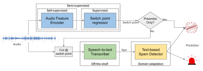
Fig 2: Phone Spam Detector Architecture
In order to cut out the preambles, we need to identify the start time in seconds of the real content where a real human answers the phone or the caller starts talking after the preamble. In machine learning terminology, this is known as the offline switch point detection (also known as changepoint/breakpoint detection) problem. The training objective is to minimize the absolute error of the predicted switch point position vs the actual.
To facilitate the analysis of sound wave data by our ML model, it needs to be preprocessed into more suitable features. In order to create compact representations of sound data, we first convert the audio recorded at a sampling rate of 22.05kHz to Mel Frequency Cepstral Coefficients (MFCC), a type of the spectrogram suitable for representing human voices, as the inputs to our encoder. (Readers can refer to this wonderful blog post for an intuitive introduction to audio processing and MFCC.) We select only phone messages longer than five seconds and limit the length of each message to a maximum of six minutes (240 seconds). Shorter audio samples are padded to 240 seconds with silence. The conversion is done using the powerful open-source Python audio processing library librosa with the length of the fast Fourier transform (FFT) windows and hop length set to 2048.

This procedure converts an audio waveform to a L x 20 MFCC matrix, where L ≤ 2584, with each window representing 93ms of audio. An example input audio waveform and its final MFCC spectrogram are shown in Fig. 3:
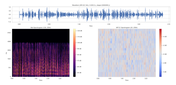
Fig 3: An example audio waveform, Mel-scale spectrogram, and MFCC matrix.
The purpose of the encoder, denoted h, is to learn an intelligent contextual representation of the input audio. The encoder is (pre-)trained with our large set of unlabeled phone messages in a self-supervised manner. This allows the encoder to learn representations of audio data in many more contexts than are available in our small labeled dataset. Similar to Wave2Vec 2.0 and OpenAI Whisper, we adopt a CNN-Transformer architecture that has shown remarkable results in various domains, including (textual) natural language processing, image recognition and speech recognition.
However, our approach differs slightly in several aspects from either of these methodologies: unlike Wave2Vec, but similar to Whisper, our encoder takes MFCC instead of raw waveform as inputs. In addition, the encoder compresses the length of the input MFCC by four times to a latent feature representation using a 1-D convolution layer with kernel size and stride equal to 4 and filter dimension 64. And the convoluted latent representation is combined with sinusoidal position embeddings and fed into a stack of four transformer blocks each with eight self-attention heads.
Thus, the whole encoder outputs contextual representations in the form of 696 64-dim vector slices known as frames – each representing 0.34 seconds of audio. During the pretraining, the encoder is topped with a deconvolution layer that projects the contextual representations to vectors of the same shape as the MFCC inputs. Given MFCC input X = (x1,…,xL), the model returns encoded feature representations Z = (z1,…,zT) where T = ⌊L/4⌋ ≤ 696. The overall structure is shown in the left figure of Fig. 4.
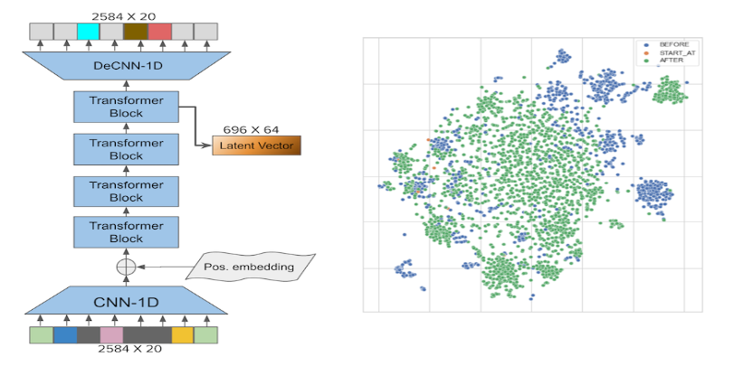
Fig 4: Audio Feature Encoder
Unlike the Whisper model, but similar to the approach taken in Wave2Vec 2.0, which trains the entire model (including the encoder) by predicting the final transcribed / translated text tokens, our self-supervised pre-training objective is to predict intermediate representations of masked positions of audio data, similar to the approach taken in Wave2Vec 2.0. However, instead of predicting the quantized latent representation as performed in Wave2Vec, our pre-trained model directly predicts the MFCC representation.
We adopt the masking strategy used in Wave2Vec and Data2Vec: sample without replacing 40% of input indices and mask up to the next 10 timesteps. In addition, we adopt the phantom masking technique used in BERT to improve robustness. Specifically, we reserve 20% of masking positions, half of which are not actually masked and the other half of which are replaced with random input slices from non-masked positions. The pretraining loss function is MSE.
We pretrain the encoder on a training set of ~50K unlabeled, randomly sampled audio recordings (corresponding to about 1300 hours of audio or 1000 hours after trimming each to the maximum length of 240 seconds) and validate using a randomly sampled validation set. The encoder is pre-trained for 200 epochs with a learning rate schedule starting at 10−5 which is increased to 10−4 after three warm-up epochs and decayed at the rate of 0.99 in the last 25 epochs. The pretraining stops early when the average validation loss of the last five epochs is worse than that of the previous five epochs.
The right figure of Fig. 5 shows the resulting t-SNE distribution of encoded contextual representations of an example audio, each slice labeled by whether it is before, at, or after the switch point. We can see clear but not crisp distinctions between slices before the switch point and those after it.
Once we transform an audio sample into a sequence of contextual latent features, we can use this sequence to predict the switch point between preamble and voice. Typically, transformer-based classifiers take the first latent vector of the variable length sequence as the feature vector and feed it to a multilayer perceptron (MLP) output layer to predict the targets. However, adopting this approach naively would result in a large mean absolute error (MAE) of 22 seconds on our hold-out validation set. This is due not only to the small size of the training set, but also to the fact that such an approach does not leverage the structure inherent in data containing meaningful switch points, specifically the property that all slices prior to the switchpoint belong to one category (the preamble) and all slices after it belong to the other (message content). We will exploit this property and leverage the information of all latent vectors as described below.
Our switch point predictor is a hybrid, multi-expert model consisting of 3 components:
Each of these components are weak experts as their accuracy metric is not superb. The model combines their opinions to produce superior predictions.
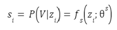
The framewise classifier takes a single frame of encoded audio latent feature, z,i , and predicts Pr(V|zi) the probability of it belonging to the voice part of the message. The classifier is parameterized by θs:
Each message has many encoded frames and we train the classifier to classify each frame independently. This increases the number of samples upon which we train thereby reducing the problem of having a small training set. For each example message in the training set, we sample with replacement 20 frames from the preambles and 30 frames from the real voice contents, resulting in over 29k preamble frames and 30k voice frames from our training set. At inference time, every frame in the message is scored by this classifier. The maximum number of scores for a message equals the maximum number of frames, which is 696.
The classifier is an MLP consisting of one 32-unit hidden layer with Guassian Error Linear Units activation, layer normalization, and a drop-out rate of 0.3, followed by a single unit output layer with sigmoid activation. The classifier is trained for 200 epochs with encoded audio features from the training set with a learning rate schedule warming up linearly from 10-6 for 10 epochs to 10−4 and then winding-down in the last 25 epochs at 0.99 decay.
Fig. 6 shows the score sequence of one example. As shown in Fig. 7, the classifier does a good job of separating the preamble from the voice though there are overlaps among their scores.
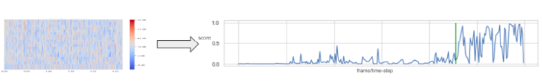
Fig 6: Score sequences. The vertical green line is the true switch point.
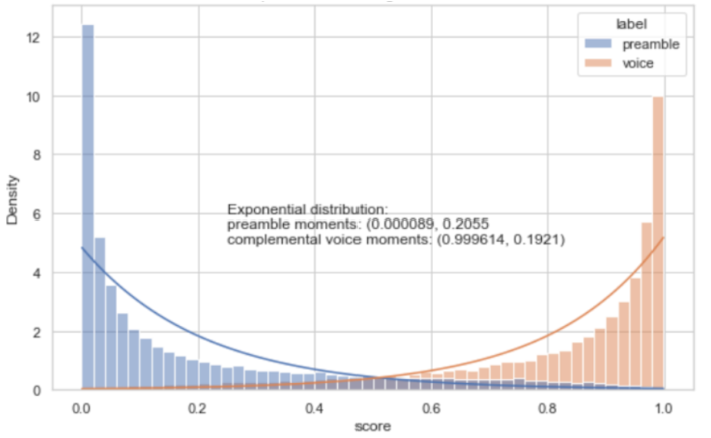
Fig 7: Preamble and voice scores PDF
Because the score sequences from the framewise classifier do not necessarily exhibit clear-cuts at the switch points, localizing the switch points is not a trivial task. We use the dynamic programming algorithm (denoted as fDYN) from the RUPTURES library to propose a set of candidate switch points K of size κ from a score sequence. This algorithm searches for segmentations of the sequence having the minimum sum of costs defined by a cost function such as the sum of point-wise L1 or L2 distances to the median values of the sequence. These candidate switch points will then be further evaluated by other experts in the framework. Note that while there is exactly one true switch point in each score sequence, specifying hyperparameter κ =1 might yield a switch point that may be far away from the true location. Instead, for the purposes of finding an appropriate yet small κ, we will define, for a given score sequence, the minimum absolute error (minAE) as the absolute distance between its true switch point to the closest candidate in K. Then, we will search for the first κ that gives a mean of minimum absolute errors (MMAE) that is less than a given threshold ζ. The κ search algorithm is shown below in Python codes in Listing 1.
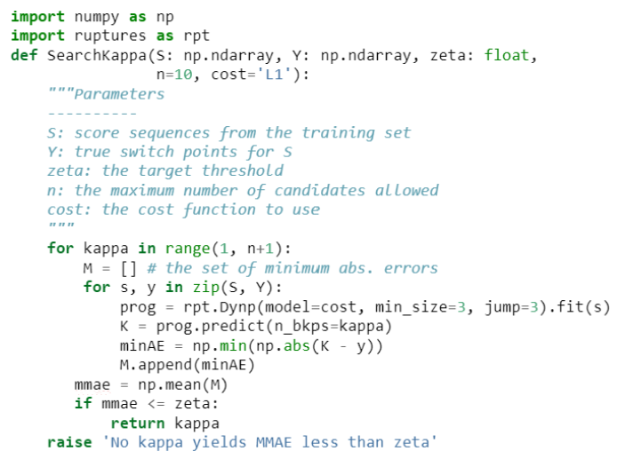
Listing 1: Search kappa the targeted number of candidate switch points to be generated
Given our training set and the target threshold ζ = 0.5, κ = 5+1, i.e. 5 switch points plus the end of the sequence (which can also be a switch point if no switch point occurs), with 0.48 seconds MMAE. Two sets of example switch point candidates are shown in Fig. 8.

Fig 8: Example switch point candidates. The orange vertical dashed lines are the candidate switch points and the green solid lines the true switch points.
The whole segment classifier takes a segment/sequence of scores si:j sliced from the original full sequence and predicts the probability Pr(V|si:j) of the whole segment being a voice segment. The classifier θws is implemented as a boosting tree, in particular a CatBoost classifier. Boosting trees are typically more data efficient than neural networks and are therefore well suited for use with our small training dataset. The classifier is trained to classify score segments to the right side of true switch points as voice and those to the left side as not voice, by minimizing binary cross entropy loss. Formally,
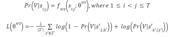
where s′ is a score sequence from the training set S′ with true switch point k′.
To avoid overfitting, we train for only 500 iterations while monitoring the validation accuracy and AUC metrics. The classifier achieves an accuracy of 0.94 and F1 score of 0.91 on the validation set.
After a given audio waveform is preprocessed to MFCC, encoded by the encoder, and scored by the framewise classifier into a sequence of scores s = (s1,…,sT), the switch point proposes a set of candidate switch points Ks = {kj}κj=1,1 ≤ kj ≤ T. Then for each candidate switch point k ∈ Ks, we produce whole segment voice classification scores for the segment of scores on each side of k, and take the ratio of the right segment probability over that of the left segment. Finally, the predicted switch point for each audio sample is the candidate with the maximum ratio. The full pipeline and combining procedure are illustrated in Fig. 9.
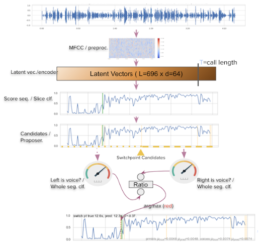
Fig 9: Full prediction pipeline and combining procedure. The orange vertical lines on the score sequence plots are the candidate switch points while the green lines are the true switch point.
Formally,
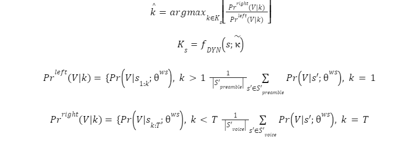
where S′preamble and S′voice are all preamble and voice segments from the training set, respectively.
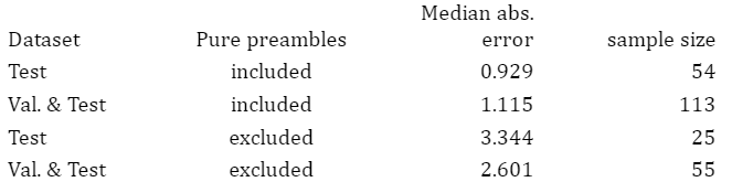
Table 1: Evaluation metrics
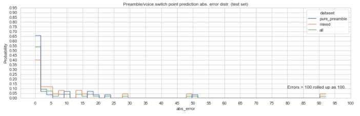
Fig 10: Switch point absolute error distribution
Table 1 shows the evaluation metrics. The detector performs very well in detecting pure preambles (which, by itself, is important as pure preamble messages account for 54% of all messages) while also performing well on messages with real contents. We choose to report median absolute errors because the distribution of the errors is skewed as shown in Fig. 10.
The previously mentioned text message spam detector is a RoBERTa model. In building that model, we adopted off-the-shelf RoBERTa parameters, pre-trained further with our internal email and text message corpus, and fine-tuned with a labeled spam message dataset. It was much easier to acquire spam labels for that task because our product includes various UI mechanisms for users to report spam messages to the platform. Versions of this model have been in production for several years.
We adopt OpenAI’s Whisper speech-to-text model for our transcription service. Whisper does an impressive job transcribing phone messages of English audio to English text, but it does make some mistakes. For example, below is a Whisper-produced transcription of a phone message, with identifiable names and phone numbers masked:

The message’s corresponding human transcription is presented below. Mistakes or discrepancies made by the Whisper ML model are highlighted in bold italic font face:
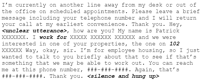
The most glaring mistake in the Whisper transcription is that the several seconds of silence after the last “thank you” gets transcribed to something that sounds like spam, despite the fact that the model does attempt to detect silence in the audio.
In spite of some mistakes, we adopt the model as is and only remove the preambles (prior to transcription) in this work. The transcribed text is then classified by the text message spam detector.
As an ablation study, we analyze the performance of our approach by using our classifier on messages transcribed with preambles retained, preambles removed by our detector, and preambles removed by a human moderator. The results are presented below:
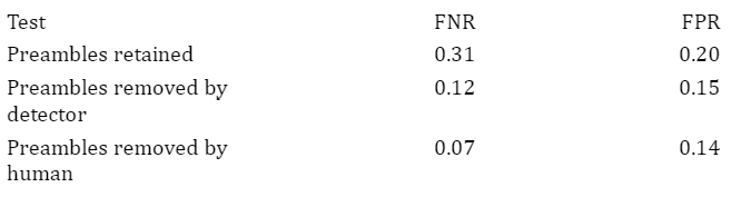
Table 2: Inference metrics
As shown in Table 2, the removal of preambles significantly improves the classification metrics. Although stripping the preamble by using our preamble detector does not provide as much lift as removing preambles by human moderation does, our automated approach still provides significant improvement over baseline and is much more scalable and efficient.
In this article, we have shown a case of detecting phone-based spam using a small labeled sample supplemented by a large easy-to-obtain, unlabeled dataset. This semi-supervised approach does not diminish the needs or benefits of collecting more labeled data. Rather, it serves as a tool in our practices of Active Learning by allowing for more accurate and efficient collection of spam samples for future model training efforts. This combination of a preamble detector trained with semi-supervised learning and off-the-shelf audio transcription and text classification models enables us to quickly start this model-data flywheel, and helps ensure the trust and safety of our users at Zillow Rentals.
