One of the core methods used within Zillow’s home recommendation engine is collaborative filtering. There are several ways collaborative filtering can be implemented. Due to the lack of explicit user ratings here at Zillow, we use matrix factorization with implicit feedback [1]. This method starts by constructing user-item interaction matrix where each entry expresses our confidence that user finds that particular item relevant. Note, that in our case items are individual listed homes. Next, we factorize this matrix into a low dimensional embedding of both users and items which together can be used to reconstruct the original interaction matrix.

Conceptually, the low-dimensional embeddings, i.e. latent home factors, should co-locate similar homes close to each other in this latent factor space. As a result, we are also planning to experiment with using this learnt home representation for recommending similar homes, e.g. by finding nearest neighbors in this latent space for each home. To increase our confidence that finding nearest neighbors in this way will lead to reasonable results, we wanted to first better understand what do these latent factors actually represent and what does this latent space look like. For instance, in the case of latent home factors, one might ask the following questions:

• What are the main home attributes that are most influential in how homes are represented in the latent space?
• Are nearby and similarly priced homes located close to each other in the latent space?

The answers to these questions are hiding somewhere in the 100+ dimensional latent factor space that is inherently difficult to visualize and comprehend. Therefore, we have tried to first project the latent factor space into an easy to understand 2D space with the help of specialized neural network architecture called Self-Organizing Map [1]. As we demonstrate in this blog post, this projection allows us to gain understanding about the relationships between explicit home attributes and latent factors. As a result, we are hoping to at least somewhat increase the interpretability of the matrix factorization model.

Collaborative Filtering Using Matrix Factorization

Collaborative Filtering (CF) as well as content based models are likely two of the most popular approaches for building a recommendation engine. When compared to the content based method, the CF method offers convenient ability to model customers’ shared interests without the need to explicitly know the attributes of the recommended items. At Zillow, due to the unique nature of our problem space where we need to recommend homes based on frequent user click patterns as well as recommend new homes that just came on the market, we leverage both content and collaborative filtering based models. As already mentioned above, in this post we will focus on the CF part of our recommendation engine.

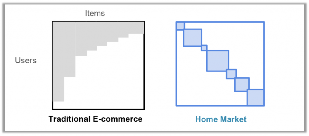
Due to the lack of explicit ratings for individual homes from our customer, we have to rely on implicit feedback, e.g. how long customers spend on the details page of each home they visited. To process this data we use the method of Implicit Matrix Factorization (IMF) for collaborative filtering [1]. To use the IMF method we build a user-item matrix where each entry represents the implicit feedback or a confidence that particular item is relevant to the user. One important and unique aspect of home recommendations is that our user-item interaction matrix is not only highly sparse but it also consists of several disjoint sub-matrices. This disjointness is due to users interacting with homes primarily in a single region where they are looking to buy a home. For example, a user who searched for homes in Seattle is very unlikely to interact with homes on the East coast in the same home search effort. Hence, due to this locale-specific interest, we apply the IMF method independently in each geographic zone instead of a single nationwide IMF model. As an illustration, the figure below shows a comparison of the user item matrix between traditional e-commerce system and a home-market system.

The goal of the IMF method is to compute a dense vector representations for each user and each item (home) that capture the key elements of a user’s preferences and the distinct nature of each home. By computing the dot product of the two latent vectors we can obtain a predicted preference values. These predicted relevance values can then be used to recommend new relevant items to each user. For model training we use the method of Alternating Least Squares (ALS), which updates the user and item vectors in alternating fashion while keeping the other fixed [1].

Self-Organizing Map

The Self-Organizing Map (SOM) algorithm was originally developed in 1981 by Teuvo Kohonen [2]. It is rather simple yet powerful modelling technique that uses unsupervised winner-takes-all competitive learning method together with cooperative adaptation to adjust itself to the topological properties of the input dataset. Typically, a SOM consists of a topological grid of neurons arranged in a 2D mesh. Because the grid of neurons is fixed and does not change during the training process, each neuron has a clearly defined spatial neighborhood. In addition to the connections to its neighboring neurons, each neuron also maintains a feature vector in the input space of the data that we are trying to model.

The training process first starts by randomly initializing all feature vectors of all neurons. Next, the network is iteratively adapted based on the training set of input data. The main step of the training process consists of randomly sampling an input feature vector, then finding its Best Matching Unit (BMU) and finally by cooperative updating of the neuron’s weight vector as well as weight vectors of its neighboring neurons in the direction of the input training data point. Here, the BMU simply refers to the neuron with the highest similarity to the input vector, e.g. having minimum Euclidean distance. This process is repeated until a prespecified convergence criteria is met, e.g. number of iteration or the cumulative sum of neurons’ weight vector updates falls below certain threshold.

To guide the training process towards convergence, the size of each BMUs’ neighborhood that is being updated is slowly decreased. This has a similar effect as for example lowering temperature during Simulated Annealing. An illustrative example of a 2D SOM with 5×5 neuron grid in the input space adapted to a 2D distribution of input data is shown in the figure below [3].

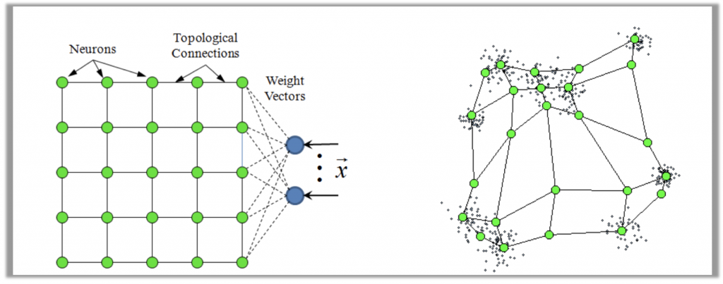
While one will unlikely want to use SOM to model 2D data, the method works in the same manner in an input space of an arbitrary dimensionality. In short, irrespective of the number of input dimensions, the organization of the neurons in the associated 2D mesh allows us to map the learnt topology back to an easy to visualize 2D space.

Visualizing Latent Home Factors using SOM

To demonstrate how we can visualize and gain understanding of the latent home factors learnt by the matrix factorization method, we created a sample dataset consisting of user-home interactions in all zip codes starting with prefix ‘98’ (i.e. most of Washington state). After applying filtering to only include users with minimum number of viewed homes, we end up with 60K frequently viewed homes. These homes correspond to individual columns in our user-item matrix. Next, we apply the ALS method to factor the matrix to a 100-dimensional latent factor representation. This means that after the matrix factorization procedure converges, we are left with 100 dimensional latent vectors for each of our 60K homes as well as 100 dimensional latent factors for all users . To implement this procedure we have used the implicit python package [4].

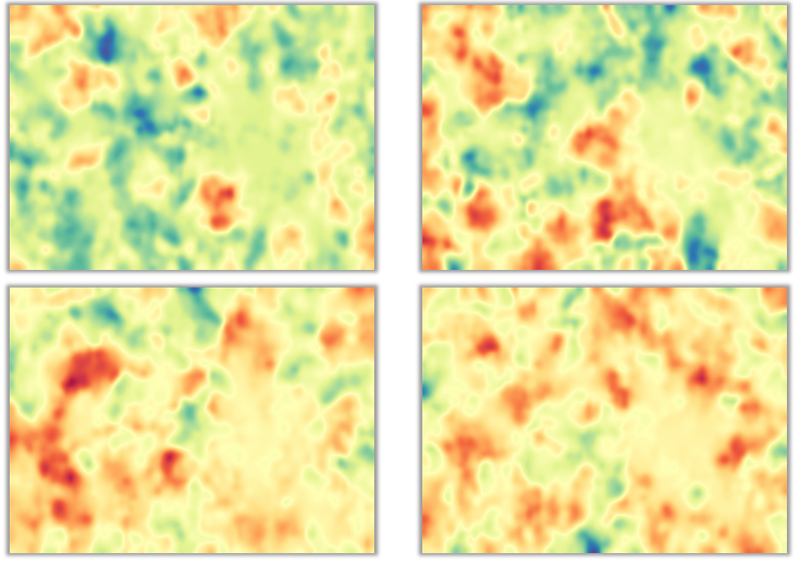
As a next step we will process this data with the help of the somoclu python package [5]. For this experiment, we have used SOM with 4000 neurons, organized in a rectangular 50×80 grid. Once the training process converges, the feature vector of each neuron approximates the distribution of similar latent home factors in the 100 dimensional input space. While this is difficult to see directly, the 2D grid structure of the SOM allows us to easily visualize this data in 2D. First we can look at each dimension separately by coloring each neuron cell with the corresponding learnt latent factor value. The figure below shows projections of 4 randomly selected latent factors projected onto the 2D SOM. By following the gradient, we can clearly see areas in the map that group vectors with similar values (e.g. continuous areas of blue corresponds to lower values and red corresponds to higher values of that specific latent factor dimension).

Unfortunately, besides nice abstract images, there is not much we can gain from these 100 different projections, one for each latent factor. Second, we can try to visualize the composite information learnt by the SOM, by rendering its so called U-Matrix. The U-Matrix encodes the distance between neighboring neurons. In the figure below, the darker the shade of blue to closer the nearby neurons are. On the other hand, the darker the shade of red, the bigger the separation between neighboring neurons in the input latent factor space. The figure on the left shows the U-Matrix for our 100-dimensional latent home factors. Clearly we can identify several areas of blue color, which likely correspond to clusters of homes with similar latent factors.

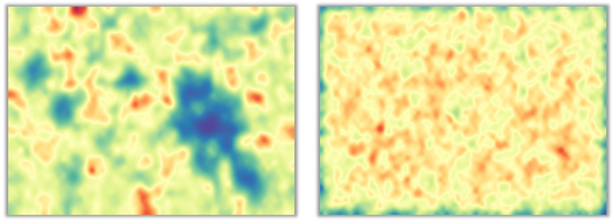
To demonstrate that there is indeed a structure in the data that is being learnt by the SOM, we have compared the U-Matrix for the latent home factors with a U-Matrix of equally sized SOM trained on randomly generated data set of the same quantity (i.e. 60K randomly sampled 100 dimensional vectors). You can see the U-Matrix in the figure above on the right. It is clearly visible, that the random U-Matrix is missing any clustering structure learnt from the data.

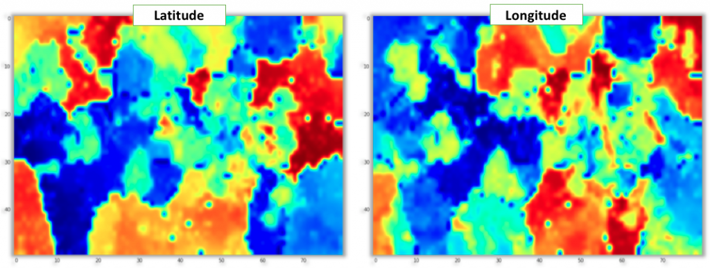
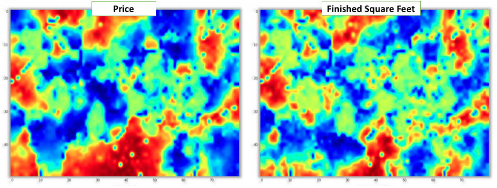
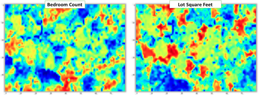
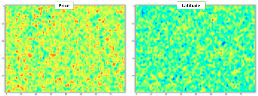
Now when we have our SOM trained in the 100 dimensional latent home factors space, we can use it to understand the relationship between explicit observable home attributes and the latent home factors learnt by the matrix factorization method. To do this, we can attach the explicit home attributes to each home (e.g. price, latitude or square footage) and then for each home find its BMU in the SOM. Finally, we can average the explicit home attribute values assigned to each BMU. When we render the interpolated values we can gain insight into how well does each explicit home attribute align with the home latent factor topology modeled by the SOM and which attributes seem to be the most influential on the latent factor space. To see this we can look at the set of six figures below that shows this projection for homes’ latitude, longitude, price, finished square footage, number of bedrooms and lot size. In general, the larger the areas/patches of similar color gradient are visible in the map, the more is that particular attribute correlated with the data distribution in the latent factor space. From the example below, we can clearly see that latitude, longitude and price appear to be aligned the most with our latent factor space since we can easily identify areas of the SOM corresponding to groupings of homes in similar geographical regions or areas grouping cheaper or more expensive homes together. While patterns are also visible for finished square footage, number of bedrooms and lot size, the relationship seems to be weaker as there are many smaller disconnected areas.

Again, to show that our SOM is really converging towards patterns in the input 100 dimensional data, we have compared the price and latitude projection from the figures above, with projection for the same attributes on top of SOM trained on random feature vectors. As can be seen below, there is no pattern visible in the SOM, as there is no relationship between the home attributes and their randomly sampled latent factors.

From the analysis above it is apparent that latitude and longitude are the most strongly correlated features with the information contained in the latent home factors. To visualize this relationship even more clearly, we have decided to try to visualize the latent factor information in a geographical space. To do this, we have trained a relatively small SOM with 4 rows of 8 neurons. The U-Matrix of the trained SOM is displayed below.

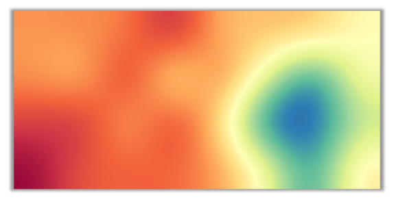
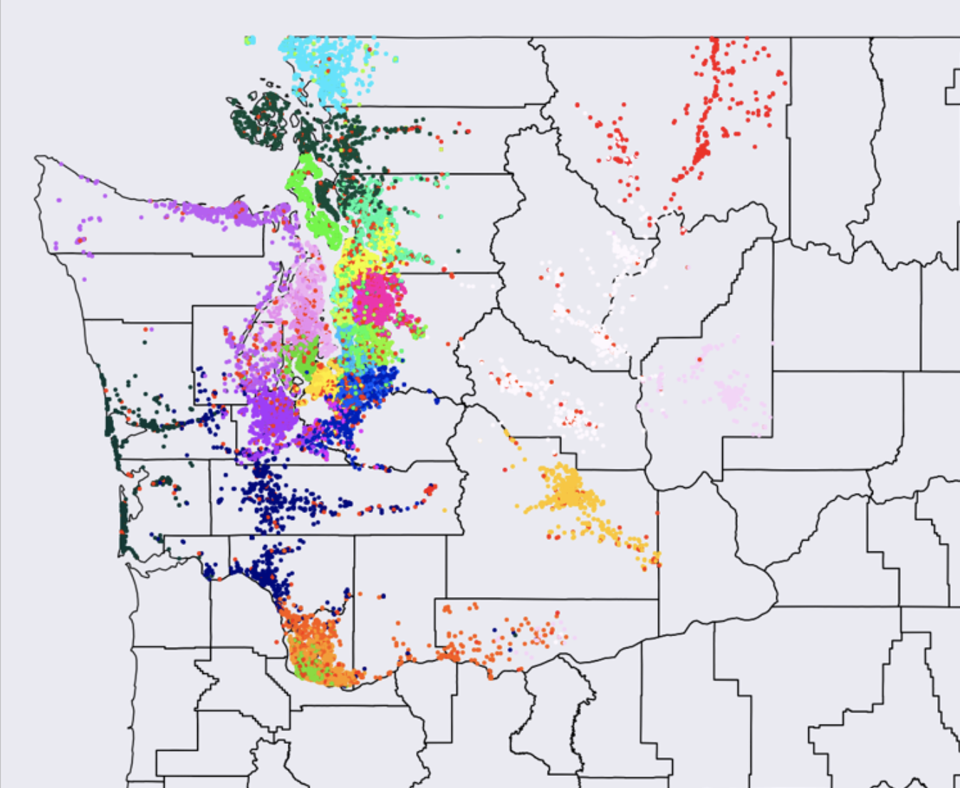
Once the SOM was trained, each of the 32 neurons can be regarded as a center of gravity of a cluster of similar latent home factors. Next, we took each home and located its BMU based on its latent factors. The index of this neuron (i.e. number between 1 and 32) was assigned to that particular home. After we annotated all homes with their BMU indexes we have plotted all homes on a map based on their latitude and longitude and we have colored their location with unique color assigned to each neuron/cluster. The result can be seen on the figure below.

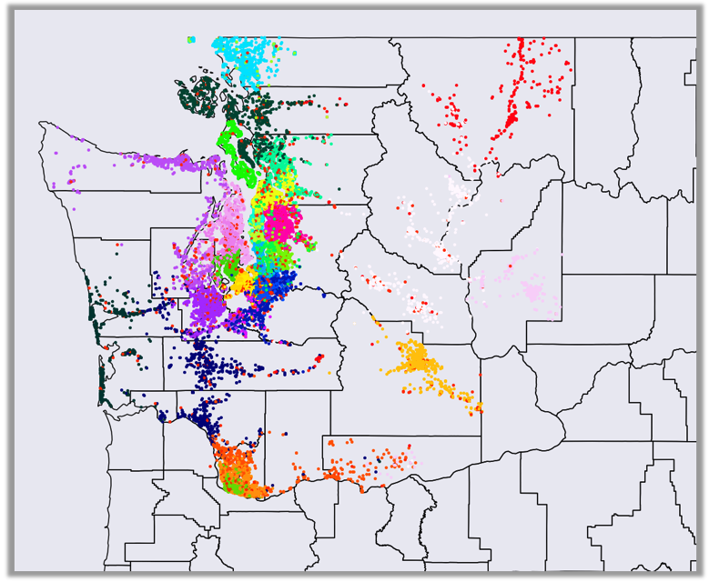
As you can see from the clustering of similarly colored points, homes assigned to the same BMU (i.e. assigned to the same cluster) are mostly collocated in the same geographical area. This clearly demonstrates that the learnt latent home factors representation is in large part driven by user home co-clicks in relatively small geographical areas (e.g. customers looking for their new home in particular city, along coast or major highways). Note that the map only shows homes in zip codes prefixed with ‘98’, which were part of our evaluation data set. Based on these insights that we were able to visually gather based on the SOM projection, we are now able to better interpret the type of information that our matrix factorization model is using to locate similar homes.  

If you find this work interesting and if you like to apply you data science and machine learning skills to our large-scale, rich and continuously evolving real-estate data set, please reach out – we are hiring.

References

[1] Y. Hu, Y. Koren, C. Volinsky, “Collaborative filtering for implicit feedback datasets”, Data Mining 2008. ICDM’08. Eighth IEEE International Conference, pp. 263-272, 2008.

[2] T. Kohonen, ―Automatic Formation of Topological Maps of Patterns in a Self-Organizing System, ‖ in Proc. SCIA, E. Oja, O. Simula, Eds. Helsinki, Finland, pp. 214-220, 1981.

[3] D. Wijayasekara, O. Linda, M. Manic, “CAVETM-SOM: Immersive Visual Data Mining Using 3D Self-Organizing Maps”, Int. Joint Conference on Neural Networks IJCNN 2011, July 31-Aug. 5, 2011.

[4] Ben Frederickson, Fast Python Collaborative Filtering for Implicit Datasets, https://pypi.org/project/implicit/

[5] Peter Wittek, Shi Chao Gao, Ik Soo Lim, Li Zhao (2017). Somoclu: An Efficient Parallel Library for Self-Organizing Maps. Journal of Statistical Software, 78(9), pp.1–21. DOI:10.18637/jss.v078.i09. arXiv:1305.1422.