There are dozens of models for the Zestimate. Many of these models require a sale transaction from the past that is adjusted forward to the price level estimate for the date of interest.

Among the models we use to accomplish this goal is the modified version of the repeat sales methodology from Case and Shiller (1987). We construct a geometric mean weighted repeat sales series. Then the WRS series is trained per county. Part of our algorithm includes filtering out outliers (not discussed in this article).

The algorithm can be broken into four phases.

Estimation

Solve for the change in prices (on the log scale) between repeat sales

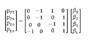
N rows, each row represents a repeat sale

T columns, each column represents the month (datekey) of a sale

Betas, model coefficients, one for each independent variable (datekey), represent the index level for the time period T normalized to the base period index level

Variables – dummy variables, where -1 represents first sale, 1 represents second sale

Fitting & Error Model

There are 3 steps part of this phase.

Step 1: Fit an OLS model to predict the log sale price delta from the transaction pair dummy matrix X (above)

log(salePrice delta) = X * Beta + e1

e1 = unobserved scalar random variables (errors)

Step 2: Fit OLS model with time between each transaction pair (delta) to squared residuals R = e12 of the transactions pairs from Step 1

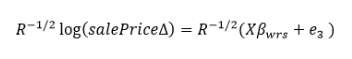
Step 3: Solve for the index levels by taking the inverse of the predicted residuals from Step 2 as weights to the formula of Step 1 via weighted least squares to solve

Imputation & Forecasting

We augment the WRS series for better accuracy. Details won’t be discussed in a later blog.

Application

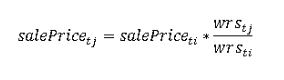
The goal again is to forward the sale price from the past to a future date. Here is the final step to convert sale price from time period i to time period j