Methodology: Zillow Rent Forecast
The Zillow Rent Index estimates median rent for a geographical region on a monthly basis. The Zillow Rent Index forecast is our prediction of ZRI over the coming year.

The Zillow Rent Index estimates median rent for a geographical region on a monthly basis. The Zillow Rent Index forecast is our prediction of ZRI over the coming year.
The Zillow Rent Index (ZRI) estimates median rent for a geographical region on a monthly basis. The Zillow Rent Forecast is our prediction of ZRI over the coming year.
We forecast ZRI for thousands of areas, at six geographic levels: ZIP code, city, county, metropolitan area, state and nation. For each region within each geography, we use a two-stage approach:
The purpose of the second step is to ensure predictions from smaller regions (e.g. states) are consistent with predictions for a larger region (e.g. nation) composed of smaller areas. Specifically, we adjust the baseline monthly predictions so the percentage change in ZRI at the larger geography is approximately equal to the weighted average of the percentage change in ZRI of the smaller geographies, where weights are determined by property counts.
Let  denote the geographic level (
 where 1=nation, 2=state, etc.). Let
  denote a region within a geographic level (
 where
where  is the number of regions in the
  geographic level, e.g.
 for the 50 states and Washington, D.C.). Let
  denote the month of the time series with
  for the current month. Let
  denote ZRI for the
  region of geographic level at month . Let
  .
.
For each region of each geography we fit an ARIMA model with parameters chosen to minimize AICc to predict baseline forecasts,  .
.
We also considered including covariates in the model, including: inventory, Zillow Home Value Index (ZHVI), median household income, unemployment rate and number of permits applied for. However, we did not find that models including covariates improved accuracy over the models without covariates.
We adapt Hyndman et al.’s approach of optimally combining forecasts for hierarchical time series in order to make our baseline forecasts “consistent” across the six geographic levels.[1] We define forecasts to be consistent when the month-over-month percentage change at a higher level (e.g. state) is approximately equal to the weighted average of the the month-over-month percentage changes at lower levels (e.g. metropolitan areas, counties, etc.) where weights are determined by property counts. The purpose of the consistency adjustment is to reconcile forecasts across the inherent geographical hierarchy of the ZRI time series: States are nested within the nation, metropolitan areas are nested within states, etc.
More formally, consistency is defined as:

for  and
and  where
where  is a noise term. The weight
  if the region of geography does not fall within the boundaries of the
  region of geography
  (e.g. the Seattle metro area has a weight of zero for all states but Washington). The non-zero weights are determined by the proportion of properties in relative to
  . We can reparametrize (1) as follows:

where  is a
is a  matrix of weights,
  is an unknown
  -vector of mean ZRI for the lowest geographic level and
  is the vector of noise terms.
Assuming  where
where  is a -vector of noise terms for the lowest geographic level, equation (2) is a linear regression model whose best linear unbiased estimator for is
  , which motivates the definition of the adjusted forecasts:

for  .
.
To examine the forecasts’ accuracy, we compare mean absolute percentage error (MAPE) to a naive model,  for . Since we have relatively short time series, we average MAPE over forecasts using 12-to-35 months of data. The percent improvement of the ARIMA models over the naive model, as well as the p-value from 2-sample paired t-tests comparing the ARIMA and naive model, are shown in the following table:
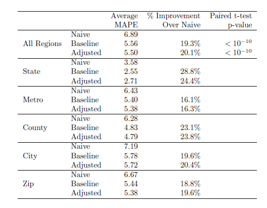 The naive forecasts were surprisingly accurate, but the ARIMA model forecasts significantly improved accuracy.
To adjust for seasonality and reduce noise in the forecast, we apply two levels of smoothing. To adjust for seasonality, we first take a 3-month moving average of each region’s forecast, then apply a Seasonal and Trend decomposition using Loess. To reduce noise in the 12-month-out forecasts and maintain consistency with the ZRI, we average the current 12-month-out seasonally-adjusted forecast with the prior two months’ seasonally-adjusted 12-month-out forecasts.
[1] Hyndman, R.J., Ahmed, R.A., Athanasopoulos, G. & Shang, H.L. (2011). Optimal combination forecasts for hierarchical time series. Computational Statistics & Data Analysis, 55(9): 2579-2589.
