This post is part one of a three-part series on now-casting the MBA Weekly Mortgage Applications Index. To read more on this subject, see the summary, part two and part three.

Each Wednesday, the Mortgage Bankers Association (MBA) reports the results of its Weekly Mortgage Applications Survey. Using the survey results, MBA creates indexes that provide information about mortgage market activity, with specific indexes for the number of fixed-rate, adjustable rate, conventional and government loans for home purchases, and mortgages refinances.[1] MBA also reports a Market Composite Index representing the entire mortgage market. As one of the higher-frequency measures of housing market activity, the survey results are viewed as a key indicator of changes in housing market conditions. Indexes are reported in seasonally adjusted (SA) and non-seasonally adjusted (NSA) levels, and as a weekly percent change. Data correspond to the week ending on Friday of the week prior to the data release (e.g., data released on Wednesday, April 2, 2014 correspond to the survey conducted during the week ending Friday, March 28, 2014).

Observers interested in estimating the MBA indexes in advance of their publication could examine a variety of variables such as interest rates that prevailed during the reference week, seasonal trends estimated from historical data, or previous values of the index assuming that lagged values of the index contain some signal about the future direction of the index. However, all of these variables are fairly indirect measures of mortgage market activity, and more directly relevant real-time data could reduce forecast error.

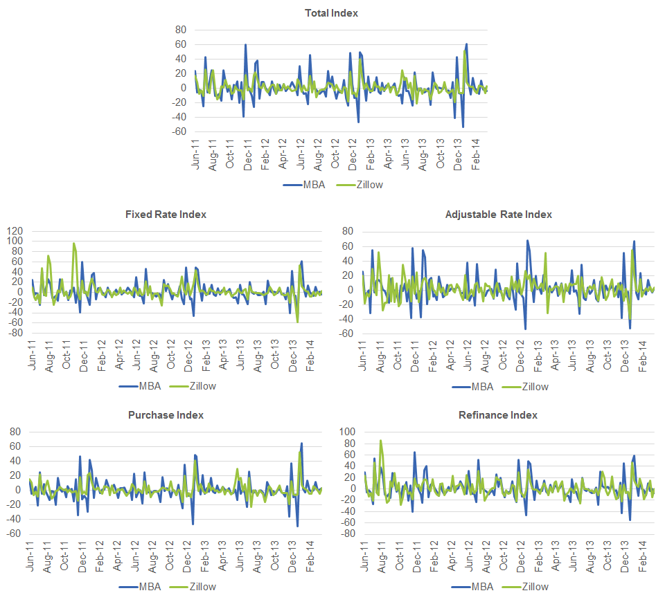
We test whether the contemporaneous count of loan requests on the Zillow Mortgage Marketplace (ZMM), known on Saturday, can help predict the MBA Mortgage Applications Index, reported the following Wednesday. The Zillow data in these models are weekly counts of loan requests for each type of mortgage on ZMM (week ending Saturday). (In part two, we discuss the explanatory power of counts of loan requests earlier in the week—for instance, the count of loan requests for each week from Sunday through Thursday.) The best performing models rely on the weekly percent change in this series. The MBA and Zillow data are aligned for each week from June 2011 through March 2014. Visual inspection of the two data sets suggest that loan requests on ZMM have some explanatory power, although the relationship is not necessarily straightforward (see charts below).

Compared to models using only information contained in previous values of the series, models using the Zillow data reduce the average error—the difference between the predicted and observed values—by roughly 40 percent, a strong improvement in the now-casts. A more comprehensive description of the methodology and the results are included below.

Detailed Methodology

The variables are defined as follows:

• is the non-seasonally adjusted value of the MBA Weekly Applications Index for mortgage product group i at time t;
• is the number of ZMM loan inquiries for mortgage product group i at time t; and
• is an indicator variable taking the value 1 if a U.S. banking holiday occurred in week t and 0 otherwise.

Where i ∈ {total, fixed rate, adjustable rate, purchase, refinance} and t represents each week ending Friday from June 3, 2011 through March 21, 2014—a total of 147 weeks. We consider models forecasting both the non-seasonally adjusted (NSA) level of the MBA Weekly Applications Index and the weekly percent change in the NSA index.[2]

For each of the MBA indexes, we compare four models:

1. A naïve forecast—that is, an AR(1) forecast including an intercept;
2. A best fit ARIMA(p,d,q) model—that is, the ARIMA(p,d,q) model automatically selected by comparing the AIC and BIC of the models;
3. A model of the MBA index as a function of a lagged value of the index and the contemporaneous weekly percent change in ZMM loan inquiries[3]; and
4. A model that includes the same explanatory variables as (3), but includes additional dummies indicating whether a U.S. banking holiday occurred the week before, of, or following the forecast week.

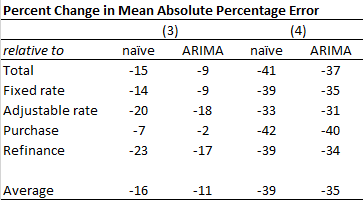
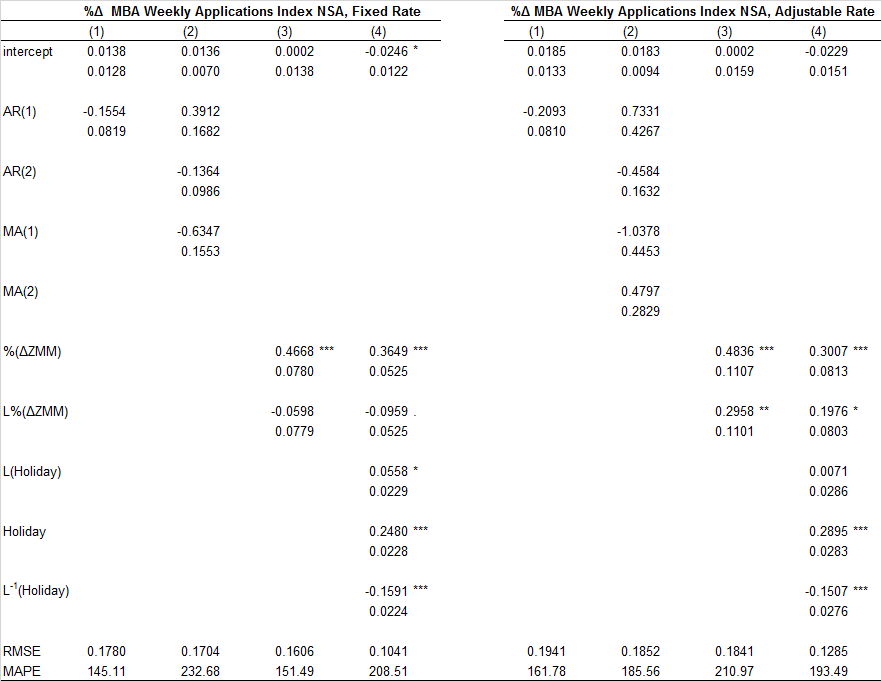
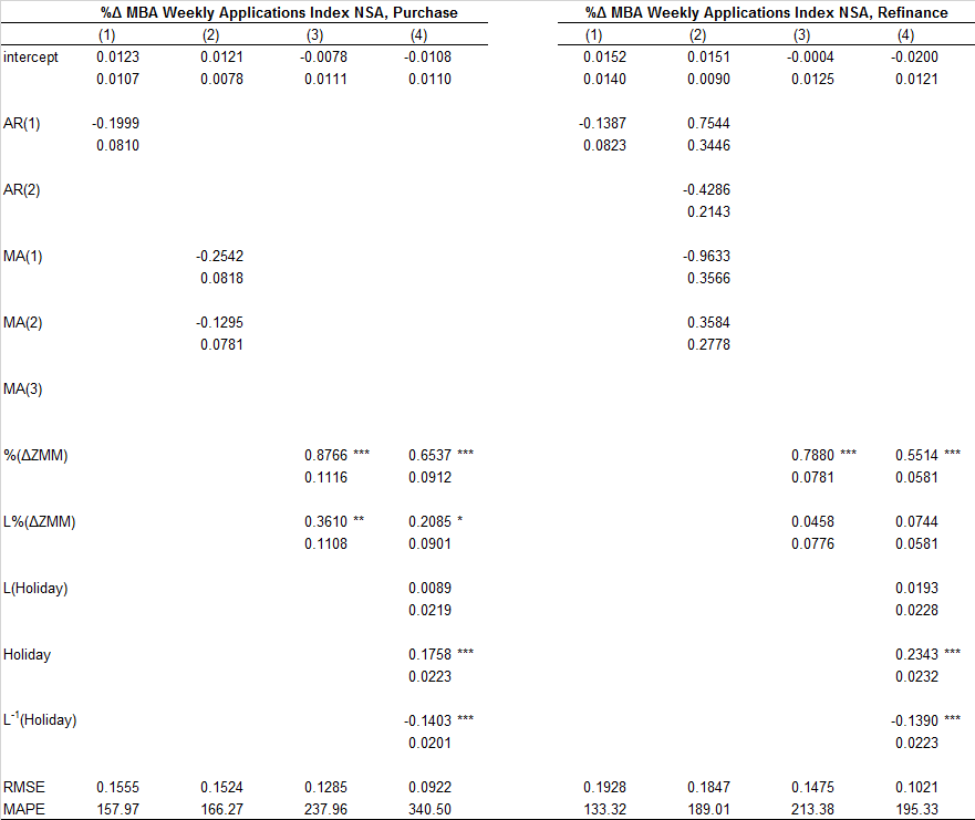
The tables below show the results of this exercise. The models perform similarly across the mortgage products, with the purchase index model having the lowest mean absolute percentage error.

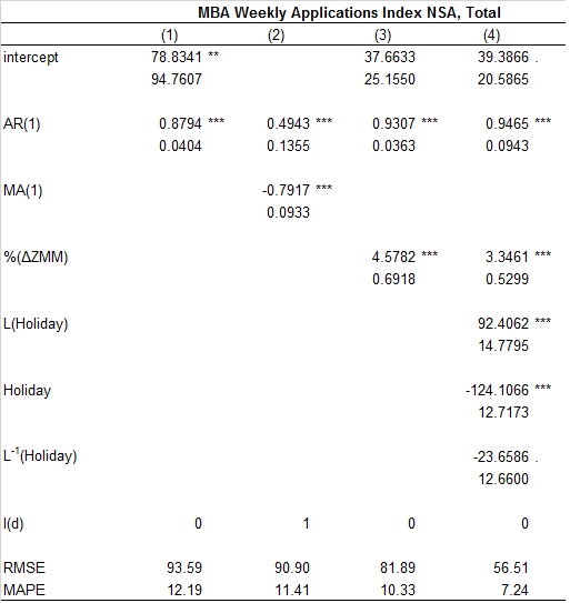
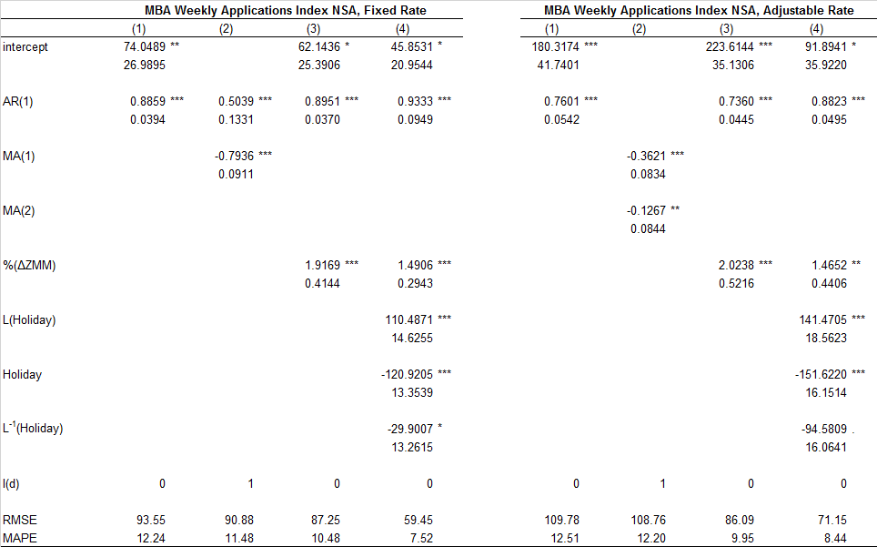
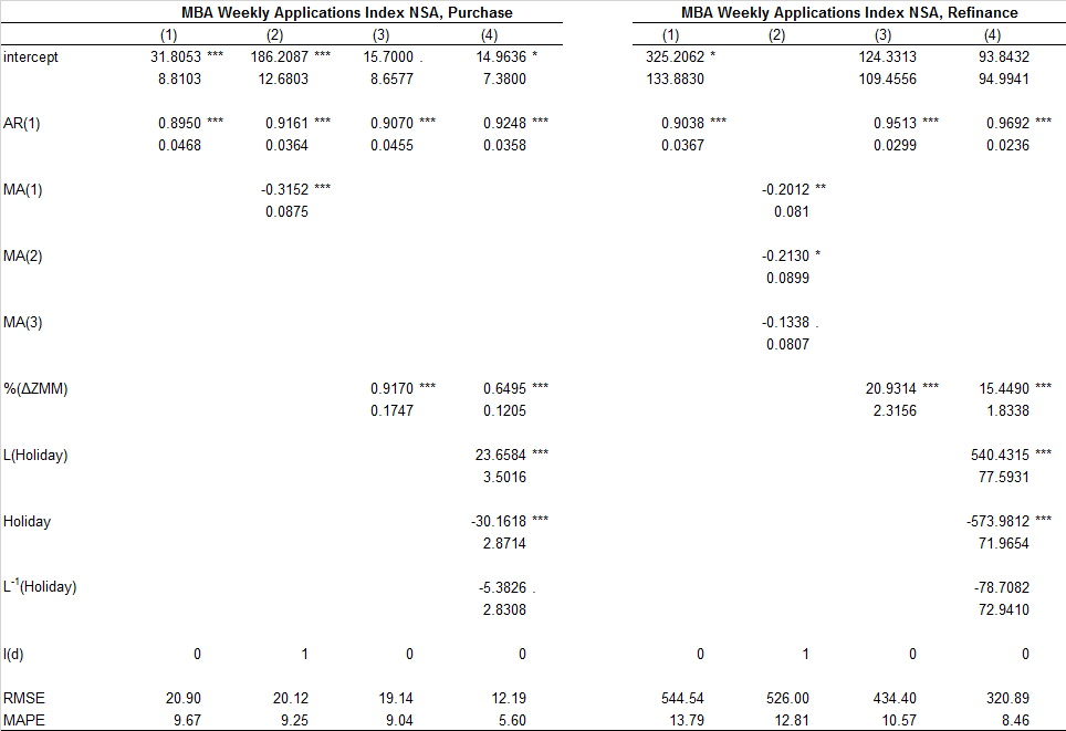
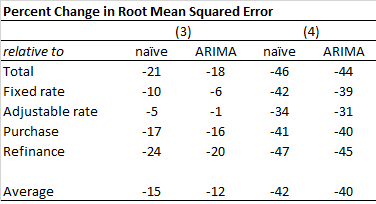
For all of the indexes, models (3) and (4) outperform the naïve and the best-fit ARIMA(p,d,q) forecasts, as illustrated in the table below. In the case of the model (3), the Root Mean Squared Error (RMSE) improves by an average of 14 percent relative to the naïve forecast and by an average of 11 percent relative to the ARIMA(p,d,q) forecast. In the case of model (4), the RMSE improves by an average of 39 percent relative to the naïve forecast and by an average of 37 percent relative to the ARIMA(p,d,q) forecast.

Next, we conduct a similar exercise to directly forecast the percent change in the MBA Weekly Mortgage Applications Index. This change is widely reported and commented on in the press as its interpretation is more intuitive than the index level. Similar to the index level forecast, we compare four models:

1. A naïve forecast—that is, an AR(1) forecast including an intercept;
2. A best fit ARIMA(p,d,q) model;
3. A model of the weekly percent change in the MBA index as function of the contemporaneous weekly percent change in ZMM loan inquiries and one lag of the percent change in ZMM loan inquiries; and
4. A model that includes the same explanatory variables as (3), but includes additional dummies indicating whether a U.S. banking holiday occurred the week before, of, or following the forecast week.

All of the models are stationary and, as a result, need no differencing to fit the ARIMA (i.e. include no I(d) terms). Similar to the results for the level series, the percent change in ZMM loan requests is significant in all of the models, and a first-order lag is significant in most. The tables below show the results modeling the weekly percent change in the total indexes.

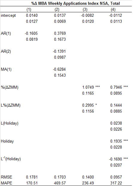
Again, models (3) and (4) outperform the naïve and the best-fit ARMA(p,q) forecasts, as illustrated in the table below. In the case of the model (3), the Root Mean Squared Error (RMSE) improves by an average of 15 percent relative to the naïve forecast and by an average of 12 percent relative to the ARMA(p,q) forecast. In the case of model (4), the RMSE improves by an average of 42 percent relative to the naïve forecast and by an average of 40 percent relative to the ARMA(p,q) forecast. These results are very similar to the results for the level index.

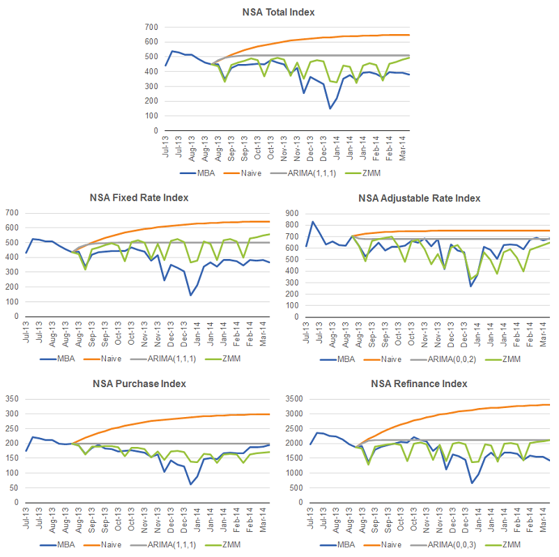
To further compare the performance of these models, we conducted in-sample and one-step-ahead tests. In-sample, the model including the percent change in ZMM loan requests term and the holiday dummies performs reasonably well over the last fifth of the sample. In the chart below, we show the results of a one-step ahead forecast over the last fifth of the sample comparing the performance of models (1), (2) and (4) with the original data for the NSA Total Index. Comparable charts for the other indices are also included below.

[1] For additional details on MBA’s Weekly Mortgage Applications Survey, see www.mbaa.org/researchandforecasts/productsandsurveys/weeklyapplicationsurvey.

[2] To ensure that the MBA Weekly Applications Index and the ZMM Loan Inquiries series are not stationary, we conduct Augmented Dickey-Fuller (ADF) tests. The results strongly reject the null hypothesis of an underlying unit root in the case of the MBA series (p-value of 0.473) and in the case of the ZMM series, although less strongly (p-value of 0.157). With the exception of NSA MBA Weekly Adjustable Rate Mortgage Index, no unit roots were detected in any of the other forecast variables.

[3] The underlying logic here is that weekly percent change in Zillow loan inquiries provides information on the change in the MBA index in a given week. If that percent change is applied to the previous value of the MBA index, we can estimate the index level for the current week.